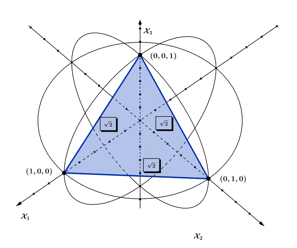
We are now able to build on the S 3 ℂ S_{3\mathbb{C}} ℂ 3 . \mathbb{C}^{3}. S 3 ℂ S_{3\mathbb{C}} l j , l_{j},
| l j | = l j ∙ l j ∗ = 1. \begin{array}{r}
\left| l_{j} \right| = \sqrt{l_{j} \bullet l_{j}^{*}} = 1.
\end{array} (1.1.96) Figure 1.1.10 – The equilateral triangle bounded by complex unit circles ∈ ℂ 3 \in \mathbb{C}^{3} We can also see that each of the vertices are separated by edge lengths equal to | 2 | \left| \sqrt{2} \right| Figure 1.1.10 1 2 ( 2 ∙ 2 ) = 1 , \frac{1}{2}\left( \sqrt{2} \bullet \sqrt{2} \right) = 1, ∈ ℂ 3 . \in \mathbb{C}^{3}.
| e i X 1 | , | e i X 2 | , | e i X 3 | = 1 , \begin{array}{r}
\left| e^{iX_{1}} \right|,\ \left| e^{iX_{2}} \right|,\left| e^{iX_{3}} \right| = 1,
\end{array} (1.1.97) where the modulus r r ℂ 3 \mathbb{C}^{3} X j X_{j}
X 1 = ( i 0 0 0 0 i 0 i 0 ) , X 2 = ( 0 0 i 0 i 0 i 0 0 ) , X 3 = ( 0 i 0 i 0 0 0 0 i ) . \begin{array}{r}
X_{1} = \begin{pmatrix}
i & 0 & 0 \\
0 & 0 & i \\
0 & i & 0
\end{pmatrix},\ \ X_{2} = \begin{pmatrix}
0 & 0 & i \\
0 & i & 0 \\
i & 0 & 0
\end{pmatrix},\ \ X_{3} = \begin{pmatrix}
0 & i & 0 \\
i & 0 & 0 \\
0 & 0 & i
\end{pmatrix}.
\end{array} (1.1.98) The real-valued elements of the group are denoted by Y j Y_{j} Y 1 Y_{1} ϵ \epsilon
Y 1 = ( 1 0 0 0 1 0 0 0 1 ) , Y 2 = ( 0 1 0 0 0 1 1 0 0 ) , Y 3 = ( 0 0 1 1 0 0 0 1 0 ) . \begin{array}{r}
Y_{1} = \begin{pmatrix}
1 & 0 & 0 \\
0 & 1 & 0 \\
0 & 0 & 1
\end{pmatrix},\ \ Y_{2} = \begin{pmatrix}
0 & 1 & 0 \\
0 & 0 & 1 \\
1 & 0 & 0
\end{pmatrix},\ \ Y_{3} = \begin{pmatrix}
0 & 0 & 1 \\
1 & 0 & 0 \\
0 & 1 & 0
\end{pmatrix}.
\end{array} (1.1.99) We define an algebra 𝔤 \mathfrak{g}
𝔤 = { X j , Y j } \begin{array}{r}
\mathfrak{g} =\left\{ X_{j},Y_{j} \right\}
\end{array} (1.1.100) Theorem (1.1.101) –The set of permutations 𝔤 ∈ U ( 3 ) \mathfrak{g} \in U(3) forms a group under composition .
Proof –
Closure → ∀ X , Y ∈ 𝔤 , X ∙ Y ∈ 𝔤 , \rightarrow \ \forall\ X,Y \in \mathfrak{g},\ \ X\ \bullet Y \in \mathfrak{g},
Associativity → ∀ X , Y , Z ∈ G , ( X ∙ Y ) ∙ Z = X ∙ ( Y ∙ Z ) , \rightarrow \ \forall\ X,Y,Z \in G,\ \ (\ X\ \bullet Y) \bullet Z = X \bullet (Y \bullet Z),
Identity → ∃ e ∈ 𝔤 : ∀ a ∈ G , a ∙ e = e ∙ a = a , \rightarrow \ \exists\ e \in \mathfrak{g}:\forall\ a \in G,\ \ a \bullet e = e \bullet a = a,
Inverse Element → ∀ a ∈ G ∃ b ∈ G : a ∙ b = b ∙ a = e . \rightarrow \forall\ a \in G\ \exists\ b \in G:\ a \bullet b = b \bullet a = e.
□ \begin{array}{r}
\ \square
\end{array} Definition (1.1.102) A finite-dimensional real or complex Lie algebra is a finite-dimensional real or complex vector space 𝔤 \mathfrak{g} , together with a Lie bracket [ X , Y ] \lbrack X,Y\rbrack , from 𝔤 × 𝔤 \mathfrak{g} \times \mathfrak{g} onto 𝔤 \mathfrak{g} , having the following properties 1
[ a X + b Y , Z ] = a [ X , Z ] + b [ Y , Z ] a n d [ Z , a X + b Y ] = a [ Z , X ] + b [ Z , Y ] ∀ X , Y , Z ∈ 𝔤 , \lbrack aX + bY,Z\rbrack = a\lbrack X,Z\rbrack + b\lbrack Y,Z\rbrack\ and\ \lbrack Z,aX + bY\rbrack = a\lbrack Z,X\rbrack + b\lbrack Z,Y\rbrack\ \forall\ X,Y,Z\ \in \ \mathfrak{g}, and for arbitrary numbers a a and b b .
[ X , Y ] = − [ Y , X ] , [ X , Z ] = − [ Z , X ] , [ Y , X ] = − [ X , Y ] , \begin{array}{r}
\lbrack X,Y\rbrack = - \lbrack Y,X\rbrack,\ \ \lbrack X,Z\rbrack = - \lbrack Z,X\rbrack,\ \ \lbrack Y,X\rbrack = - \lbrack X,Y\rbrack,\
\end{array}
The Jacobi identity holds:
[ X , [ Y , Z ] ] + [ Z , [ X , Y ] ] + [ Y , [ Z , X ] ] = 0 , ∀ X , Y , Z ∈ 𝔤 . \begin{array}{r}
\left\lbrack X,\lbrack Y,Z\rbrack \right\rbrack + \left\lbrack Z,\lbrack X,Y\rbrack \right\rbrack + \left\lbrack Y,\lbrack Z,X\rbrack \right\rbrack = 0,\ \forall\ X,Y,Z\ \in \ \mathfrak{g}.
\end{array} Theorem (1.1.103) –The set of permutations 𝔤 = { X j , Y j } \ \mathfrak{g} =\left\{ X_{j},Y_{j} \right\} forms a finite-dimensional complex Lie algebra over a complex vector space.
Proof – The Lie Algebra Definition
Bilinearity: [ a X + b Y , Z ] = a [ X , Z ] + b [ Y , Z ] \ \lbrack aX + bY,Z\rbrack = a\lbrack X,Z\rbrack + b\lbrack Y,Z\rbrack and [ Z , a X + b Y ] = a [ Z , X ] + b [ Z , Y ] ∀ X , Y , Z ∈ \lbrack Z,aX + bY\rbrack = a\lbrack Z,X\rbrack + b\lbrack Z,Y\rbrack\ \forall\ X,Y,Z\ \in 𝔤 \mathfrak{g}
and for arbitrary numbers a a n d b a\ and\ b ,
[ X , Y ] = − [ Y , X ] ∀ \lbrack X,Y\rbrack = - \lbrack Y,X\rbrack\ \forall X , Y ∈ 𝔤 X,Y \in \mathfrak{g} ,
The Jacobi Identity holds:
[ X , [ Y , Z ] ] + [ Y , [ Z , X ] ] + [ Z , [ X , Y ] ] = 0 , \left\lbrack X,\lbrack Y,Z\rbrack \right\rbrack + \left\lbrack Y,\lbrack Z,X\rbrack \right\rbrack + \left\lbrack Z,\lbrack X,Y\rbrack \right\rbrack = 0, ∀ X , Y ∈ 𝔤 \forall\ X,Y \in \mathfrak{g}
□ \square Taking the exponential mapping of our Lie algebra elements ∈ 𝔤 \in \mathfrak{g}
G = e 𝔤 = { e X j , e Y j } , \begin{array}{r}
G = e^{\mathfrak{g}} = \left\{ e^{X_{j}},e^{Y_{j}} \right\},
\end{array} (1.1.104) we can define that a matrix Lie group by exponentiation is a smooth manifold over G G
Definition (1.1.105) The Unitary Group 𝐔 ( 𝟑 ) \mathbf{U}\left( \mathbf{3} \right) is a group under composition, sitting in the complex geometric space ℂ 3 × 3 \mathbb{C}^{3 \times 3}
U ( 3 ) = { G ∈ ℂ 3 × 3 : G ∗ G = I , | det ( G ) | = I } , \begin{array}{r}
U(3) = \left\{ G \in \mathbb{C}^{3 \times 3}:G^{*}G = I,\left| \det(G) \right| = I \right\},
\end{array} with a set of Lie algebra elements 𝔤 = { X j , Y j } \mathfrak{g} =\left\{ X_{j},Y_{j} \right\} , for angle arguments x j , y j ∈ ℝ x_{j},y_{j}\in \mathbb{R}
𝔤 = { ( i x 1 0 0 0 0 i x 1 0 i x 1 0 ) , ( 0 0 i x 2 0 i x 2 0 i x 2 0 0 ) , ( 0 i x 3 0 i x 3 0 0 0 0 i x 3 ) , ( y 1 0 0 0 y 1 0 0 0 y 1 ) , ( 0 y 2 0 0 0 y 2 y 2 0 0 ) , ( 0 0 y 3 y 3 0 0 0 y 3 0 ) } . \begin{array}{r}
\mathfrak{g} =\left\{ \begin{array}{r}
\begin{pmatrix}
ix_{1} & 0 & 0 \\
0 & 0 & ix_{1} \\
0 & ix_{1} & 0
\end{pmatrix},\ \ \ \begin{pmatrix}
0 & 0 & ix_{2} \\
0 & ix_{2} & 0 \\
ix_{2} & 0 & 0
\end{pmatrix},\ \ \ \begin{pmatrix}
0 & ix_{3} & 0 \\
ix_{3} & 0 & 0 \\
0 & 0 & ix_{3}
\end{pmatrix}, \\
\begin{pmatrix}
y_{1} & 0 & 0 \\
0 & y_{1} & 0 \\
0 & 0 & y_{1}
\end{pmatrix},\ \ \ \begin{pmatrix}
0 & y_{2} & 0 \\
0 & 0 & y_{2} \\
y_{2} & 0 & 0
\end{pmatrix},\ \ \ \begin{pmatrix}
0 & 0 & y_{3} \\
y_{3} & 0 & 0 \\
0 & y_{3} & 0
\end{pmatrix}
\end{array} \right\}.
\end{array} (1.1.106) The set of rotation matrices G = { e X j , e Y j } G = \left\{ e^{X_{j}},e^{Y_{j}} \right\} ± ∠ a r g u m e n t s ∈ ℝ \pm \ \angle\ arguments\in \mathbb{R} e X j e^{X_{j}}
G X 1 : { G X 1 ( x 1 ) = ( e i x 1 0 0 0 cos ( x 1 ) i s i n ( x 1 ) 0 i s i n ( x 1 ) cos ( x 1 ) ) , G X 1 ( − x 1 ) = ( e − i x 1 0 0 0 cos ( x 1 ) − i s i n ( x 1 ) 0 − i s i n ( x 1 ) cos ( x 1 ) ) } , \begin{array}{r}
{G_{X}}_{1}:\left\{ {G_{X}}_{1}\left( x_{1} \right) = \begin{pmatrix}
e^{ix_{1}} & 0 & 0 \\
0 & \cos\left( x_{1} \right) & isin\left( x_{1} \right) \\
0 & isin\left( x_{1} \right) & \cos\left( x_{1} \right)
\end{pmatrix},\ \ {G_{X}}_{1}\left( {- x}_{1} \right) = \begin{pmatrix}
e^{- ix_{1}} & 0 & 0 \\
0 & \cos\left( x_{1} \right) & - isin\left( x_{1} \right) \\
0 & - isin\left( x_{1} \right) & \cos\left( x_{1} \right)
\end{pmatrix} \right\},
\end{array} (1.1.107) G X 2 : { G X 2 ( x 2 ) = ( cos ( x 2 ) 0 i s i n ( x 2 ) 0 e i x 2 0 i s i n ( x 2 ) 0 cos ( x 2 ) ) , G X 2 ( − x 2 ) = ( cos ( x 2 ) 0 − i s i n ( x 2 ) 0 e − i x 2 0 − i s i n ( x 2 ) 0 cos ( x 2 ) ) } , \begin{array}{r}
{G_{X}}_{2}:\left\{ {G_{X}}_{2}\left( x_{2} \right) = \begin{pmatrix}
\cos\left( x_{2} \right) & 0 & isin\left( x_{2} \right) \\
0 & e^{ix_{2}} & 0 \\
isin\left( x_{2} \right) & 0 & \cos\left( x_{2} \right)
\end{pmatrix},\ \ {G_{X}}_{2}\left( {- x}_{2} \right) = \begin{pmatrix}
\cos\left( x_{2} \right) & 0 & - isin\left( x_{2} \right) \\
0 & e^{- ix_{2}} & 0 \\
- isin\left( x_{2} \right) & 0 & \cos\left( x_{2} \right)
\end{pmatrix} \right\},
\end{array} (1.1.108) G X 3 : { G X 3 ( x 3 ) = ( cos ( x 3 ) i s i n ( x 3 ) 0 i s i n ( x 3 ) cos ( x 3 ) 0 0 0 e i x 3 ) , G X 3 ( − x 3 ) = ( − cos ( x 3 ) − i s i n ( x 3 ) 0 i s i n ( x 3 ) cos ( x 3 ) 0 0 0 e − i x 3 ) } . \begin{array}{r}
{G_{X}}_{3}:\left\{ {G_{X}}_{3}\left( x_{3} \right) = \begin{pmatrix}
\cos\left( x_{3} \right) & isin\left( x_{3} \right) & 0 \\
isin\left( x_{3} \right) & \cos\left( x_{3} \right) & 0 \\
0 & 0 & e^{ix_{3}}
\end{pmatrix},\ \ {G_{X}}_{3}\left( {- x}_{3} \right) = \left( - \begin{matrix}
\cos\left( x_{3} \right) & - isin\left( x_{3} \right) & 0 \\
isin\left( x_{3} \right) & \cos\left( x_{3} \right) & 0 \\
0 & 0 & e^{- ix_{3}}
\end{matrix} \right) \right\}.
\end{array} (1.1.109) The non-identity cyclic permutation elements take on a more complicated form with exponentiation. Effectively, the exponential series e i x e^{ix} three-way trigonometric functions in more depth in later sections. To be complete, we present the Lie groups G Y 2 {G_{Y}}_{2} G Y 3 {G_{Y}}_{3}
G Y 2 : { G Y 2 ( y 2 ) = ( e y 2 3 + 2 3 e − y 2 2 cos ( 3 y 2 2 ) e y 2 3 − 2 3 e − y 2 2 sin ( π 6 + 3 y 2 2 ) e y 2 3 − 2 3 e − y 2 2 sin ( π 6 − 3 y 2 2 ) e y 2 3 − 2 3 e − y 2 2 sin ( π 6 − 3 y 2 2 ) e y 2 3 + 2 3 e − y 2 2 cos ( 3 y 2 2 ) e y 2 3 − 2 3 e − y 2 2 sin ( π 6 + 3 y 2 2 ) e y 2 3 − 2 3 e − y 2 2 sin ( π 6 + 3 y 2 2 ) e y 2 3 − 2 3 e − y 2 2 sin ( π 6 − 3 y 2 2 ) e y 2 3 + 2 3 e − y 2 2 cos ( 3 y 2 2 ) ) , G Y 2 ( − y 2 ) = ( e − y 2 3 + 2 3 e y 2 2 cos ( 3 y 2 2 ) e − y 2 3 − 2 3 e y 2 2 sin ( π 6 − 3 y 2 2 ) e − y 2 3 − 2 3 e y 2 2 sin ( π 6 + 3 y 2 2 ) e − y 2 3 − 2 3 e y 2 2 sin ( π 6 + 3 y 2 2 ) e − y 2 3 + 2 3 e y 2 2 cos ( 3 y 2 2 ) e − y 2 3 − 2 3 e y 2 2 sin ( π 6 − 3 y 2 2 ) e − y 2 3 − 2 3 e y 2 2 sin ( π 6 − 3 y 2 2 ) e − y 2 3 − 2 3 e y 2 2 sin ( π 6 + 3 y 2 2 ) e − y 2 3 + 2 3 e y 2 2 cos ( 3 y 2 2 ) ) } ( 1.1.110 ) \begin{array}{r}
G_{Y_{2}}:\left\{ \begin{array}{r}
G_{Y_{2}}\left( y_{2} \right) = \begin{pmatrix}
\frac{e^{y_{2}}}{3} + \frac{2}{3}e^{- \frac{y_{2}}{2}}\cos\left( \frac{\sqrt{3}y_{2}}{2} \right) & \frac{e^{y_{2}}}{3} - \frac{2}{3}e^{- \frac{y_{2}}{2}}\sin\left( \frac{\pi}{6} + \frac{\sqrt{3}y_{2}}{2} \right) & \frac{e^{y_{2}}}{3} - \frac{2}{3}e^{- \frac{y_{2}}{2}}\sin\left( \frac{\pi}{6} - \frac{\sqrt{3}y_{2}}{2} \right) \\
\frac{e^{y_{2}}}{3} - \frac{2}{3}e^{- \frac{y_{2}}{2}}\sin\left( \frac{\pi}{6} - \frac{\sqrt{3}y_{2}}{2} \right) & \frac{e^{y_{2}}}{3} + \frac{2}{3}e^{- \frac{y_{2}}{2}}\cos\left( \frac{\sqrt{3}y_{2}}{2} \right) & \frac{e^{y_{2}}}{3} - \frac{2}{3}e^{- \frac{y_{2}}{2}}\sin\left( \frac{\pi}{6} + \frac{\sqrt{3}y_{2}}{2} \right) \\
\frac{e^{y_{2}}}{3} - \frac{2}{3}e^{- \frac{y_{2}}{2}}\sin\left( \frac{\pi}{6} + \frac{\sqrt{3}y_{2}}{2} \right) & \frac{e^{y_{2}}}{3} - \frac{2}{3}e^{- \frac{y_{2}}{2}}\sin\left( \frac{\pi}{6} - \frac{\sqrt{3}y_{2}}{2} \right) & \frac{e^{y_{2}}}{3} + \frac{2}{3}e^{- \frac{y_{2}}{2}}\cos\left( \frac{\sqrt{3}y_{2}}{2} \right)
\end{pmatrix}, \\
G_{Y_{2}}\left( {- y}_{2} \right) = \begin{pmatrix}
\frac{e^{{- y}_{2}}}{3} + \frac{2}{3}e^{\frac{y_{2}}{2}}\cos\left( \frac{\sqrt{3}y_{2}}{2} \right) & \frac{e^{- y_{2}}}{3} - \frac{2}{3}e^{\frac{y_{2}}{2}}\sin\left( \frac{\pi}{6} - \frac{\sqrt{3}y_{2}}{2} \right) & \frac{e^{{- y}_{2}}}{3} - \frac{2}{3}e^{\frac{y_{2}}{2}}\sin\left( \frac{\pi}{6} + \frac{\sqrt{3}y_{2}}{2} \right) \\
\frac{e^{{- y}_{2}}}{3} - \frac{2}{3}e^{\frac{y_{2}}{2}}\sin\left( \frac{\pi}{6} + \frac{\sqrt{3}y_{2}}{2} \right) & \frac{e^{{- y}_{2}}}{3} + \frac{2}{3}e^{\frac{y_{2}}{2}}\cos\left( \frac{\sqrt{3}y_{2}}{2} \right) & \frac{e^{- y_{2}}}{3} - \frac{2}{3}e^{\frac{y_{2}}{2}}\sin\left( \frac{\pi}{6} - \frac{\sqrt{3}y_{2}}{2} \right) \\
\frac{e^{- y_{2}}}{3} - \frac{2}{3}e^{\frac{y_{2}}{2}}\sin\left( \frac{\pi}{6} - \frac{\sqrt{3}y_{2}}{2} \right) & \frac{e^{{- y}_{2}}}{3} - \frac{2}{3}e^{\frac{y_{2}}{2}}\sin\left( \frac{\pi}{6} + \frac{\sqrt{3}y_{2}}{2} \right) & \frac{e^{{- y}_{2}}}{3} + \frac{2}{3}e^{\frac{y_{2}}{2}}\cos\left( \frac{\sqrt{3}y_{2}}{2} \right)
\end{pmatrix}
\end{array} \right\}(1.1.110)
\end{array} G Y 3 : { G Y 3 ( y 3 ) = ( e y 3 3 + 2 3 e − y 3 2 cos ( 3 y 3 2 ) e y 3 3 − 2 3 e − y 3 2 sin ( π 6 − 3 y 3 2 ) e y 3 3 − 2 3 e − y 3 2 sin ( π 6 + 3 y 3 2 ) e y 3 3 − 2 3 e − y 3 2 sin ( π 6 + 3 y 3 2 ) e y 3 3 + 2 3 e − y 3 2 cos ( 3 y 3 2 ) e y 3 3 − 2 3 e − y 3 2 sin ( π 6 − 3 y 3 2 ) e y 3 3 − 2 3 e − y 3 2 sin ( π 6 − 3 y 3 2 ) e y 3 3 − 2 3 e − y 3 2 sin ( π 6 + 3 y 3 2 ) e y 3 3 + 2 3 e − y 3 2 cos ( 3 y 3 2 ) ) , G Y 3 ( − y 3 ) = ( e − y 3 3 + 2 3 e y 3 2 cos ( 3 y 3 2 ) e − y 3 3 − 2 3 e y 3 2 sin ( π 6 + 3 y 3 2 ) e − y 3 3 − 2 3 e y 3 2 sin ( π 6 − 3 y 3 2 ) e − y 3 3 − 2 3 e y 3 2 sin ( π 6 − 3 y 3 2 ) e − y 3 3 + 2 3 e y 3 2 cos ( 3 y 3 2 ) e − y 3 3 − 2 3 e y 3 2 sin ( π 6 + 3 y 3 2 ) e − y 3 3 − 2 3 e y 3 2 sin ( π 6 + 3 y 3 2 ) e − y 3 3 − 2 3 e y 3 2 sin ( π 6 − 3 y 3 2 ) e − y 3 3 + 2 3 e y 3 2 cos ( 3 y 3 2 ) ) } ( 1.1.111 ) G_{Y_{3}}:\left\{ \begin{array}{r}
G_{Y_{3}}\left( y_{3} \right) = \begin{pmatrix}
\frac{e^{y_{3}}}{3} + \frac{2}{3}e^{- \frac{y_{3}}{2}}\cos\left( \frac{\sqrt{3}y_{3}}{2} \right) & \frac{e^{y_{3}}}{3} - \frac{2}{3}e^{- \frac{y_{3}}{2}}\sin\left( \frac{\pi}{6} - \frac{\sqrt{3}y_{3}}{2} \right) & \frac{e^{y_{3}}}{3} - \frac{2}{3}e^{- \frac{y_{3}}{2}}\sin\left( \frac{\pi}{6} + \frac{\sqrt{3}y_{3}}{2} \right) \\
\frac{e^{y_{3}}}{3} - \frac{2}{3}e^{- \frac{y_{3}}{2}}\sin\left( \frac{\pi}{6} + \frac{\sqrt{3}y_{3}}{2} \right) & \frac{e^{y_{3}}}{3} + \frac{2}{3}e^{- \frac{y_{3}}{2}}\cos\left( \frac{\sqrt{3}y_{3}}{2} \right) & \frac{e^{y_{3}}}{3} - \frac{2}{3}e^{- \frac{y_{3}}{2}}\sin\left( \frac{\pi}{6} - \frac{\sqrt{3}y_{3}}{2} \right) \\
\frac{e^{y_{3}}}{3} - \frac{2}{3}e^{- \frac{y_{3}}{2}}\sin\left( \frac{\pi}{6} - \frac{\sqrt{3}y_{3}}{2} \right) & \frac{e^{y_{3}}}{3} - \frac{2}{3}e^{- \frac{y_{3}}{2}}\sin\left( \frac{\pi}{6} + \frac{\sqrt{3}y_{3}}{2} \right) & \frac{e^{y_{3}}}{3} + \frac{2}{3}e^{- \frac{y_{3}}{2}}\cos\left( \frac{\sqrt{3}y_{3}}{2} \right)
\end{pmatrix}, \\
G_{Y_{3}}\left( {- y}_{3} \right) = \begin{pmatrix}
\frac{e^{{- y}_{3}}}{3} + \frac{2}{3}e^{\frac{y_{3}}{2}}\cos\left( \frac{\sqrt{3}y_{3}}{2} \right) & \frac{e^{- y_{3}}}{3} - \frac{2}{3}e^{\frac{y_{3}}{2}}\sin\left( \frac{\pi}{6} + \frac{\sqrt{3}y_{3}}{2} \right) & \frac{e^{{- y}_{3}}}{3} - \frac{2}{3}e^{\frac{y_{3}}{2}}\sin\left( \frac{\pi}{6} - \frac{\sqrt{3}y_{3}}{2} \right) \\
\frac{e^{{- y}_{3}}}{3} - \frac{2}{3}e^{\frac{y_{3}}{2}}\sin\left( \frac{\pi}{6} - \frac{\sqrt{3}y_{3}}{2} \right) & \frac{e^{{- y}_{3}}}{3} + \frac{2}{3}e^{\frac{y_{3}}{2}}\cos\left( \frac{\sqrt{3}y_{3}}{2} \right) & \frac{e^{- y_{3}}}{3} - \frac{2}{3}e^{\frac{y_{3}}{2}}\sin\left( \frac{\pi}{6} + \frac{\sqrt{3}y_{3}}{2} \right) \\
\frac{e^{- y_{3}}}{3} - \frac{2}{3}e^{\frac{y_{3}}{2}}\sin\left( \frac{\pi}{6} + \frac{\sqrt{3}y_{3}}{2} \right) & \frac{e^{{- y}_{3}}}{3} - \frac{2}{3}e^{\frac{y_{3}}{2}}\sin\left( \frac{\pi}{6} - \frac{\sqrt{3}y_{3}}{2} \right) & \frac{e^{{- y}_{3}}}{3} + \frac{2}{3}e^{\frac{y_{3}}{2}}\cos\left( \frac{\sqrt{3}y_{3}}{2} \right)
\end{pmatrix}
\end{array} \right\}(1.1.111) We can see the resemblance the G X j G_{X_{j}} R x , R y , R z R_{x},\ R_{y},\ R_{z} S O ( 3 ) SO(3)
G x = ( 0 0 0 0 0 − 1 0 1 0 ) , G y = ( 0 0 1 0 0 0 − 1 0 0 ) , G z = ( 0 − 1 0 1 0 0 0 0 0 ) . \begin{array}{r}
G_{x} = \begin{pmatrix}
0 & 0 & 0 \\
0 & 0 & - 1 \\
0 & 1 & 0
\end{pmatrix},\ \ G_{y} = \begin{pmatrix}
0 & 0 & 1 \\
0 & 0 & 0 \\
- 1 & 0 & 0
\end{pmatrix},\ \ G_{z} = \begin{pmatrix}
0 & - 1 & 0 \\
1 & 0 & 0 \\
0 & 0 & 0
\end{pmatrix}.
\end{array} (1.1.112) An element of S O ( 3 ) SO(3)
α 1 G x + α 2 G y + α 3 G z ∈ S O ( 3 ) , α j ∈ ℝ 3 . \begin{array}{r}
\alpha_{1}G_{x} + \alpha_{2}G_{y} + \alpha_{3}G_{z} \in SO(3),\ \ \ \alpha_{j} \in \mathbb{R}^{3}.
\end{array} (1.1.113) Exponentiation of the G j G_{j}
R x = ( 1 0 0 0 cos ( α ) − sin ( α ) 0 sin ( α ) cos ( α ) ) , R y = ( cos ( α ) 0 sin ( α ) 0 1 0 ) − sin ( α ) 0 cos ( α ) ) , R z = ( cos ( α ) − sin ( α ) 0 sin ( α ) cos ( α ) 0 0 0 1 ) . \begin{array}{r}
R_{x} = \begin{pmatrix}
1 & 0 & 0 \\
0 & \cos(\alpha) & - \sin(\alpha) \\
0 & \sin(\alpha) & \cos(\alpha)
\end{pmatrix},\ \ \ R_{y} = \begin{pmatrix}
\cos(\alpha) & 0 & \sin(\alpha) \\
0 & 1 & 0) \\
- \sin(\alpha) & 0 & \cos(\alpha)
\end{pmatrix},\ \ \ R_{z} = \begin{pmatrix}
\cos(\alpha) & - \sin(\alpha) & 0 \\
\sin(\alpha) & \cos(\alpha) & 0 \\
0 & 0 & 1
\end{pmatrix}.
\end{array} (1.1.114) With our U ( 3 ) U(3) ℝ 3 \mathbb{R}^{3} ℂ 3 \mathbb{C}^{3} X 1 X_{1} R x ∈ S O ( 3 ) R_{x} \in SO(3) 𝐞 𝐢 𝐗 𝟏 \mathbf{e}^{\mathbf{i}\mathbf{X}_{\mathbf{1}}} X 2 X 3 ∈ ℂ 2 X_{2}X_{3} \in \mathbb{C}^{2}
e X 1 = ( 𝐞 𝐢 𝐗 𝟏 0 0 0 cos ( X 1 ) i s i n ( X 1 ) 0 i s i n ( X 1 ) cos ( X 1 ) ) . \begin{array}{r}
e^{X_{1}} = \begin{pmatrix}
\mathbf{e}^{\mathbf{i}\mathbf{X}_{\mathbf{1}}} & 0 & 0 \\
0 & \cos\left( X_{1} \right) & isin\left( X_{1} \right) \\
0 & isin\left( X_{1} \right) & \cos\left( X_{1} \right)
\end{pmatrix}.
\end{array} (1.1.115) By taking the complex modulus of 𝐞 𝐢 𝐗 𝟏 \mathbf{e}^{\mathbf{i}\mathbf{X}_{\mathbf{1}}} i ≅ ( 0 ∓ 1 ± 1 0 ) i \cong \begin{pmatrix}
0 & \mp 1 \\
\pm 1 & 0
\end{pmatrix} ℝ 3 \mathbb{R}^{3} ℂ 3 \mathbb{C}^{3}
e X 1 = ( | 𝐞 𝐢 𝐗 𝟏 | 0 0 0 cos ( X 1 ) i s i n ( X 1 ) 0 i s i n ( X 1 ) cos ( X 1 ) ) ℂ 3 → ℝ 3 → ( 1 0 0 0 cos ( X 1 ) ∓ sin ( X 1 ) 0 ± sin ( X 1 ) cos ( X 1 ) ) . \begin{array}{r}
e^{X_{1}} = \begin{pmatrix}
\left| \mathbf{e}^{\mathbf{i}\mathbf{X}_{\mathbf{1}}} \right| & 0 & 0 \\
0 & \cos\left( X_{1} \right) & isin\left( X_{1} \right) \\
0 & isin\left( X_{1} \right) & \cos\left( X_{1} \right)
\end{pmatrix}\mathbb{C}^{3} \rightarrow \mathbb{R}^{3} \rightarrow \begin{pmatrix}
1 & 0 & 0 \\
0 & \cos\left( X_{1} \right) & \mp \sin\left( X_{1} \right) \\
0 & {\pm \sin}\left( X_{1} \right) & \cos\left( X_{1} \right)
\end{pmatrix}.
\end{array} (1.1.116) The similarities between our exponentiated X j X_{j} S O ( 3 ) SO(3) ) begets the question, is the three-dimensional space we are all familiar with actually ℂ 3 \mathbb{C}^{3} U ( 1 ) U(1) S O ( 2 ) SO(2) U ( 3 ) U(3) X j X_{j} ∈ ℂ 3 \in \mathbb{C}^{3} X j X_{j} X j X_{j} X k X l X_{k}X_{l} Eq. 1.1.116 𝐞 𝐢 𝐗 𝟏 \mathbf{e}^{\mathbf{i}\mathbf{X}_{\mathbf{1}}} ∈ ℂ , \in \mathbb{C}, ℂ 2 \mathbb{C}^{2} X 2 / X 3 . X_{2}{/X}_{3}. 𝔤 \mathfrak{g}
𝔤 = V D V − 1 . \begin{array}{r}
\mathfrak{g} =VDV^{- 1}.
\end{array} (1.1.117) The algebra set 𝔤 = { X j , Y j } \mathfrak{g} =\left\{ X_{j},Y_{j} \right\}
𝔤 = { ( y 1 0 0 0 y 1 0 0 0 y 1 ) ( x 1 y 2 + x 3 y 3 + x 2 y 3 + x 3 x 2 y 2 + x 1 y 2 + x 2 y 3 + x 1 x 3 ) } . \begin{array}{r}
\mathfrak{g} =\left\{ \begin{pmatrix}
y_{1} & 0 & 0 \\
0 & y_{1} & 0 \\
0 & 0 & y_{1}
\end{pmatrix}\begin{pmatrix}
x_{1} & {y_{2} + x}_{3} & y_{3} + x_{2} \\
{y_{3} + x}_{3} & x_{2} & {y_{2} + x}_{1} \\
{y_{2} + x}_{2} & {y_{3} + x}_{1} & x_{3}
\end{pmatrix} \right\}.
\end{array} (1.1.118) In the eigendecomposition 𝔤 = Y 1 ( V D V − 1 ) \mathfrak{g} =Y_{1}\left( VDV^{- 1} \right) Y 1 Y_{1} V D V − 1 VDV^{- 1} e 1 e^{1} D , V D,V
D = ( − ( ℛ 2 ) − 𝛌 2 0 0 0 − ( ℛ 2 ) + 𝛌 𝟐 0 0 0 ℛ + 𝛄 ) , \begin{array}{r}
D = \begin{pmatrix}
- \left( \frac{\mathcal{R}}{2} \right) - \frac{\mathbf{\lambda}}{2} & 0 & 0 \\
0 & - \left( \frac{\mathcal{R}}{2} \right) + \frac{\mathbf{\lambda}}{\mathbf{2}} & 0 \\
0 & 0 & \ \mathcal{R} +\mathbf{\gamma}
\end{pmatrix},
\end{array} (1.1.119) V = ( ( y 2 − y 3 − 2 x 1 + 2 x 3 + 𝛌 2 ( x 1 − x 2 − y 2 + y 3 ) ) − ( y 2 − y 3 − 2 x 1 + 2 x 3 + 𝛌 2 ( x 1 − x 2 − y 2 + y 3 ) ) 1 − ( y 2 − y 3 − 2 x 1 + 2 x 3 + 𝛌 2 ( x 1 − x 2 − y 2 + y 3 ) ) ( y 2 − y 3 − 2 x 1 + 2 x 3 + 𝛌 2 ( x 1 − x 2 − y 2 + y 3 ) ) 1 1 1 1 ) , \begin{array}{r}
V = \begin{pmatrix}
\left( \frac{y_{2} - y_{3} - 2x_{1} + 2x_{3} + \mathbf{\lambda}}{2\left( x_{1} - x_{2} - y_{2} + y_{3} \right)} \right) & - \left( \frac{y_{2} - y_{3} - 2x_{1} + 2x_{3} + \mathbf{\lambda}}{2\left( x_{1} - x_{2} - y_{2} + y_{3} \right)} \right) & 1 \\
- \left( \frac{y_{2} - y_{3} - 2x_{1} + 2x_{3} + \mathbf{\lambda}}{2\left( x_{1} - x_{2} - y_{2} + y_{3} \right)} \right) & \left( \frac{y_{2} - y_{3} - 2x_{1} + 2x_{3} + \mathbf{\lambda}}{2\left( x_{1} - x_{2} - y_{2} + y_{3} \right)} \right) & 1 \\
1 & 1 & \ 1
\end{pmatrix},
\end{array} (1.1.120) for ℛ = ( y 2 + y 3 ) \mathcal{R} =\left( y_{2} + y_{3} \right) γ = ( x 1 + x 2 + x 3 ) , 𝛌 = − 3 y 2 2 + 6 y 2 y 3 − 3 y 3 2 + 4 x 1 2 − 4 x 1 x 2 − 4 x 1 x 3 + 4 x 2 2 − 4 x 2 x 3 + 4 x 3 2 . \ \ \gamma = \left( x_{1} + x_{2} + x_{3} \right),\ \ \mathbf{\lambda} = \ \sqrt{\begin{array}{r}
- 3y_{2}^{2} + 6y_{2}y_{3} - 3y_{3}^{2} + 4x_{1}^{2} \\
- 4x_{1}x_{2} - 4x_{1}x_{3} + 4x_{2}^{2} - 4x_{2}x_{3} + 4x_{3}^{2}
\end{array}}.
We can take advantage of the diagonalized form to calculate the polar form of the entire group
G = V e D V − 1 , \begin{array}{r}
G = Ve^{D}V^{- 1},
\end{array} (1.1.121) finding the matrix representation G = e y 1 ( V e D V − 1 ) G = e^{y_{1}}\left( Ve^{D}V^{- 1} \right)
e y 1 ( e ( γ + ℛ ) 3 + e − ℛ 2 ( 2 cosh ( 𝛌 2 ) 3 − i ∂ 𝛌 ∂ X 1 sinh ( 𝛌 2 ) 3 ) e ( γ + ℛ ) 3 − e − ℛ 2 ( cosh ( 𝛌 2 ) 3 + ∂ 𝛌 ∂ Y 2 + i ∂ 𝛌 ∂ X 3 sinh ( 𝛌 2 ) 3 ) e ( γ + ℛ ) 3 − e − ℛ 2 ( cosh ( 𝛌 2 ) 3 + − ∂ 𝛌 ∂ Y 3 − i ∂ 𝛌 ∂ X 2 sinh ( 𝛌 2 ) 3 ) e ( γ + ℛ ) 3 − e − ℛ 2 ( cosh ( 𝛌 2 ) 3 + − ∂ 𝛌 ∂ Y 3 − i ∂ 𝛌 ∂ X 3 sinh ( 𝛌 2 ) 3 ) e ( γ + ℛ ) 3 + e − ℛ 2 ( 2 cosh ( 𝛌 2 ) 3 − i ∂ 𝛌 ∂ X 2 sinh ( 𝛌 2 ) 3 ) e ( γ + ℛ ) 3 − e − ℛ 2 ( cosh ( 𝛌 2 ) 3 + ∂ 𝛌 ∂ Y 2 + i ∂ 𝛌 ∂ X 1 sinh ( 𝛌 2 ) 3 ) e ( γ + ℛ ) 3 − e − ℛ 2 ( cosh ( 𝛌 2 ) 3 + ∂ 𝛌 ∂ Y 2 + i ∂ 𝛌 ∂ X 2 sinh ( 𝛌 2 ) 3 ) e ( γ + ℛ ) 3 − e − ℛ 2 ( cosh ( 𝛌 2 ) 3 + − ∂ 𝛌 ∂ Y 3 − i ∂ 𝛌 ∂ X 1 sinh ( 𝛌 2 ) 3 ) e ( γ + ℛ ) 3 + e − ℛ 2 ( 2 cosh ( 𝛌 2 ) 3 − i ∂ 𝛌 ∂ X 3 sinh ( 𝛌 2 ) 3 ) ) \begin{array}{r}
e^{y_{1}}\begin{pmatrix}
\frac{e^{\left( \gamma+ \mathcal{R} \right)}}{3} + e^{- \frac{\mathcal{R}}{2}}\left( \frac{2\cosh\left( \frac{\mathbf{\lambda}}{2} \right)}{3} - \frac{i\frac{\partial\mathbf{\lambda}}{\partial X_{1}}\sinh\left( \frac{\mathbf{\lambda}}{2} \right)}{3} \right) & \frac{e^{\left( \gamma+ \mathcal{R} \right)}}{3} - e^{- \frac{\mathcal{R}}{2}}\left( \frac{\cosh\left( \frac{\mathbf{\lambda}}{2} \right)}{3} + \frac{\frac{\partial\mathbf{\lambda}}{\partial Y_{2}} + i\frac{\partial\mathbf{\lambda}}{\partial X_{3}}\sinh\left( \frac{\mathbf{\lambda}}{2} \right)}{3} \right) & \frac{e^{\left( \gamma+ \mathcal{R} \right)}}{3} - e^{- \frac{\mathcal{R}}{2}}\left( \frac{\cosh\left( \frac{\mathbf{\lambda}}{2} \right)}{3} + \frac{- \frac{\partial\mathbf{\lambda}}{\partial Y_{3}} - i\frac{\partial\mathbf{\lambda}}{\partial X_{2}}\sinh\left( \frac{\mathbf{\lambda}}{2} \right)}{3} \right) \\
\frac{e^{\left( \gamma+ \mathcal{R} \right)}}{3} - e^{- \frac{\mathcal{R}}{2}}\left( \frac{\cosh\left( \frac{\mathbf{\lambda}}{2} \right)}{3} + \frac{- \frac{\partial\mathbf{\lambda}}{\partial Y_{3}} - i\frac{\partial\mathbf{\lambda}}{\partial X_{3}}\sinh\left( \frac{\mathbf{\lambda}}{2} \right)}{3} \right) & \frac{e^{\left( \gamma+ \mathcal{R} \right)}}{3} + e^{- \frac{\mathcal{R}}{2}}\left( \frac{2\cosh\left( \frac{\mathbf{\lambda}}{2} \right)}{3} - \frac{i\frac{\partial\mathbf{\lambda}}{\partial X_{2}}\sinh\left( \frac{\mathbf{\lambda}}{2} \right)}{3} \right) & \frac{e^{\left( \gamma+ \mathcal{R} \right)}}{3} - e^{- \frac{\mathcal{R}}{2}}\left( \frac{\cosh\left( \frac{\mathbf{\lambda}}{2} \right)}{3} + \frac{\frac{\partial\mathbf{\lambda}}{\partial Y_{2}} + i\frac{\partial\mathbf{\lambda}}{\partial X_{1}}\sinh\left( \frac{\mathbf{\lambda}}{2} \right)}{3} \right) \\
\frac{e^{\left( \gamma+ \mathcal{R} \right)}}{3} - e^{- \frac{\mathcal{R}}{2}}\left( \frac{\cosh\left( \frac{\mathbf{\lambda}}{2} \right)}{3} + \frac{\frac{\partial\mathbf{\lambda}}{\partial Y_{2}} + i\frac{\partial\mathbf{\lambda}}{\partial X_{2}}\sinh\left( \frac{\mathbf{\lambda}}{2} \right)}{3} \right) & \frac{e^{\left( \gamma+ \mathcal{R} \right)}}{3} - e^{- \frac{\mathcal{R}}{2}}\left( \frac{\cosh\left( \frac{\mathbf{\lambda}}{2} \right)}{3} + \frac{- \frac{\partial\mathbf{\lambda}}{\partial Y_{3}} - i\frac{\partial\mathbf{\lambda}}{\partial X_{1}}\sinh\left( \frac{\mathbf{\lambda}}{2} \right)}{3} \right) & \frac{e^{\left( \gamma+ \mathcal{R} \right)}}{3} + e^{- \frac{\mathcal{R}}{2}}\left( \frac{2\cosh\left( \frac{\mathbf{\lambda}}{2} \right)}{3} - \frac{i\frac{\partial\mathbf{\lambda}}{\partial X_{3}}\sinh\left( \frac{\mathbf{\lambda}}{2} \right)}{3} \right)
\end{pmatrix}
\end{array} Figure 1.1.11 The Complete G = e y 1 ( V e D V − 1 ) G = e^{y_{1}}\left( Ve^{D}V^{- 1} \right) Lie Group Representation for partial derivatives ∂ 𝛌 ∂ 𝐗 𝐣 \frac{\partial\mathbf{\lambda}}{\partial\mathbf{X}_{\mathbf{j}}}
∂ 𝛌 ∂ 𝐗 𝟏 = ( 2 x 1 − x 2 − x 3 ) 𝛌 , ∂ 𝛌 ∂ 𝐗 𝟐 = ( − x 1 + 2 x 2 − x 3 ) 𝛌 , ∂ 𝛌 ∂ 𝐗 𝟑 = ( − x 1 − x 2 + 2 x 3 ) 𝛌 . \begin{array}{r}
\frac{\partial\mathbf{\lambda}}{\partial\mathbf{X}_{\mathbf{1}}} = \frac{\left( 2x_{1} - x_{2} - x_{3} \right)}{\mathbf{\lambda}},\ \ \ \frac{\partial\mathbf{\lambda}}{\partial\mathbf{X}_{\mathbf{2}}} = \frac{\left( - x_{1} + 2x_{2} - x_{3} \right)}{\mathbf{\lambda}},\ \ \ \frac{\partial\mathbf{\lambda}}{\ \partial\mathbf{X}_{\mathbf{3}}} = \frac{\left( - x_{1} - x_{2} + 2x_{3} \right)}{\mathbf{\lambda}}.
\end{array} It is also noted that for the polar form of the group G , G,
G ∗ G = I , \begin{array}{r}
G^{*}G = I,
\end{array} (1.1.122) and
det ( G ) = e ( i x 1 + i x 2 + i x 3 ) ∴ | det ( G ) | = I . \begin{array}{r}
\det(G) = e^{\left( ix_{1} + ix_{2} + ix_{3} \right)}\therefore|\det(G)|\ = I.
\end{array} (1.1.123) In the U ( 3 ) U(3) S 3 S_{3} ℂ 3 \mathbb{C}^{3} ∈ ℂ 3 \in \mathbb{C}^{3}