Masteries · Jason GlowneyArithmoí Book 1

Masteries

1.1.27 Projective Forms

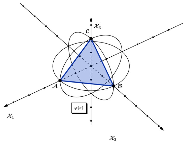
In this sec­tion, we will use the ex­am­ple of the S3ℂ/D3ℂS_{3\mathbb{C}}/D_{3\mathbb{C}} group and its el­e­ments to in­ves­ti­gate the ex­po­nen­tial map onto U(3).U(3).By ex­po­nen­ti­a­tion, we take the simple ro­ta­tions and re­flec­tions of the Lie al­ge­bra el­e­ments and trans­form these into a con­tin­u­ous man­i­fold in ℂ3\mathbb{C}^{3} space. In layper­son's terms, we are taking the group el­e­ments from ro­tat­ing/re­flect­ing the tri­an­gle's ver­tices to an in­fi­nite number of po­ten­tial vertex points aligned with the com­plex axes. This makes it pos­si­ble to rotate and re­flect con­tin­u­ous­ly to any points in the ℂ3\mathbb{C}^{3} space. Again, we show in Figure 1.1.20 below, the iden­ti­ty ϵ\epsilon ori­ent­ed along the pos­i­tive real axes for our equi­lat­er­al tri­an­gle ABCABC.

Figure
Figure 1.1.20 –The ϕ(ϵ)\phi(\epsilon) map­ping for S3ℂ/D3ℂS_{3\mathbb{C}}/D_{3\mathbb{C}}.

When con­sid­er­ing per­mu­ta­tions in matrix form, we can gain more geo­met­ric in­sight when com­pared to per­mu­ta­tions de­pict­ed in two-rowed forms. To clar­i­fy the rep­re­sen­ta­tion of per­mu­ta­tions in these stan­dard forms, we denote the X1X_{1} per­mu­ta­tion from S3ℂ/D3ℂS_{3\mathbb{C}}/D_{3\mathbb{C}} in a two-rowed per­mu­ta­tion form as

X1=(i0000i0i0)→(iAiBiCiAiCiB),\begin{array}{r} X_{1} = \begin{pmatrix} i & 0 & 0 \\ 0 & 0 & i \\ 0 & i & 0 \end{pmatrix}\mathbf{\rightarrow}\begin{pmatrix} iA & iB & iC \\ iA & iC & iB \end{pmatrix}\mathbf{,} \end{array}
(1.1.206)

where we have re­flect­ed the second and third el­e­ments, while keep­ing the first fixed. Al­though it is clear to see what is hap­pen­ing in the two-rowed per­mu­ta­tion no­ta­tion, we are miss­ing that any ro­ta­tion or re­flec­tion occurs in some geo­met­ric space. In the Xj,YjX_{j},Y_{j} matrix no­ta­tion, it is well-de­fined that we are using ma­tri­ces in a ℂ3\mathbb{C}^{3} geo­met­ric space. The entry X1(1,1)X_{1}(1,1) is the axis and re­mains fixed, while there is a re­flec­tion in the X2/X3X_{2}/X_{3}-plane that is rep­re­sent­ed by the 2×22 \times 2 matrix in the bottom-right corner. The crit­i­cal point to re­al­ize is these are Lie al­ge­bra gen­er­a­tors ori­ent­ed in a geo­met­ric space.

Figure
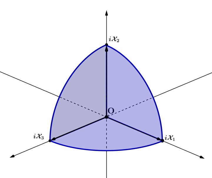
Figure 1.1.21 – Pos­i­tive-Imag­i­nary Axes of S3ℂ/D3ℂS_{3\mathbb{C}}/D_{3\mathbb{C}}.

In Figure 1.1.21, we rep­re­sent the S3ℂ/D3ℂS_{3\mathbb{C}}/D_{3\mathbb{C}} group's pos­i­tive imag­i­nary axes in three di­men­sions to orient the ob­serv­er. We define a pos­i­tive ro­ta­tion as a coun­ter­clock­wise linear trans­for­ma­tion, which im­plies the iX2iX_{2}-axis is lo­cat­ed coun­ter­clock­wise from iX1iX_{1}, for iX3iX_{3} de­fined as the axis of ro­ta­tion, and the iX3iX_{3} axis is lo­cat­ed clock­wise from the iX1iX_{1} axis for iX2iX_{2}, de­fined as the axis of ro­ta­tion. To remind the reader, the Xj,YjX_{j},Y_{j}-type per­mu­ta­tions are shown again below

X1=(i0000i0i0),  X2=(00i0i0i00),  X3=(0i0i0000i),\begin{array}{r} X_{1} = \begin{pmatrix} i & 0 & 0 \\ 0 & 0 & i \\ 0 & i & 0 \end{pmatrix},\ \ X_{2} = \begin{pmatrix} 0 & 0 & i \\ 0 & i & 0 \\ i & 0 & 0 \end{pmatrix},\ \ X_{3} = \begin{pmatrix} 0 & i & 0 \\ i & 0 & 0 \\ 0 & 0 & i \end{pmatrix}, \end{array}
(1.1.207)
Y1=(100010001),  Y2=(010001100),  Y3=(001100010).\begin{array}{r} Y_{1} = \begin{pmatrix} 1 & 0 & 0 \\ 0 & 1 & 0 \\ 0 & 0 & 1 \end{pmatrix},\ \ Y_{2} = \begin{pmatrix} 0 & 1 & 0 \\ 0 & 0 & 1 \\ 1 & 0 & 0 \end{pmatrix},\ \ Y_{3} = \begin{pmatrix} 0 & 0 & 1 \\ 1 & 0 & 0 \\ 0 & 1 & 0 \end{pmatrix}. \end{array}
(1.1.208)

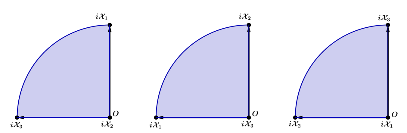
We can rep­re­sent the XjX_{j} per­mu­ta­tion el­e­ments as ori­entable forms, where the matrix entry along the main di­ag­o­nal is the fixed axis for each el­e­ment and can be thought of as a vector on its tail, coming out of the page. We rep­re­sent this in Figure 1.1.22 using points going from left to right to rep­re­sent iX3,iX2,iX1iX_{3},iX_{2},iX_{1}, as seen on the bottom-right of each form.

Figure
Figure 1.1.22 - Pro­jec­tive forms for Xj∈S3ℂ/D3ℂX_{j} \in S_{3\mathbb{C}}/D_{3\mathbb{C}}.

The other two vec­tors are pro­ject­ed in the re­spec­tive XjX_{j}-planes, point­ing up for the pos­i­tive/coun­ter­clock­wise ori­en­ta­tion and to the left for the neg­a­tive/clock­wise ori­en­ta­tion. Fur­ther, we can rep­re­sent the XjX_{j} per­mu­ta­tion el­e­ments in no­ta­tion to en­com­pass this, where ⨀\mathbf{\bigodot} sig­ni­fies the vector or­thog­o­nal to the pro­ject­ed form, ↺\circlearrowleft as the axis which is ori­ent­ed coun­ter­clock­wise from ⨀\mathbf{\bigodot}, and ↻\circlearrowright as the axis ori­ent­ed clock­wise from ⨀\mathbf{\bigodot}. Using this no­ta­tion, the Lie al­ge­bras can be rep­re­sent­ed in the fol­low­ing matrix forms

X1=(⨀0000↺0↻0),  X2=(00↻0⨀0↺00),  X3=(0↺0↻0000⨀).\begin{array}{r} X_{1} = \begin{pmatrix} \mathbf{\bigodot} & 0 & 0 \\ 0 & 0 & \circlearrowleft \\ 0 & \circlearrowright & 0 \end{pmatrix},\ \ X_{2} = \begin{pmatrix} 0 & 0 & \circlearrowright \\ 0 & \mathbf{\bigodot} & 0 \\ \circlearrowleft & 0 & 0 \end{pmatrix}\mathbf{,\ \ }X_{3} = \begin{pmatrix} 0 & \circlearrowleft & 0 \\ \circlearrowright & 0 & 0 \\ 0 & 0 & \mathbf{\bigodot} \end{pmatrix}\mathbf{.} \end{array}
(1.1.209)

The reader may recall, the columns in ma­tri­ces rep­re­sent the vec­tors in the xjx_{j} di­rec­tions, while the rows of the ma­tri­ces are the xkx_{k} com­po­nents of each column vector. So, taking the per­mu­ta­tion X3X_{3} as an ex­am­ple, we have

iX3(3,3)=(0i0i0000i)→the x3 component of the x3 vector,{iX}_{3}(3,3) = \begin{pmatrix} 0 & i & 0 \\ i & 0 & 0 \\ 0 & 0 & \boxed{i} \end{pmatrix} \rightarrow the\ x_{3}\ component\ of\ the\ x_{3}\ vector,
iX3(1,2)=(0i0i0000i)→the x1 component of the x2 vector,{iX}_{3}(1,2) = \begin{pmatrix} 0 & \boxed{i} & 0 \\ i & 0 & 0 \\ 0 & 0 & i \end{pmatrix} \rightarrow the\ x_{1}\ component\ of\ the\ x_{2}\ vector,
iX3(2,1)=(0i0i0000i)→the x2 component of the x1 vector.\begin{array}{r} iX_{3}(2,1) = \begin{pmatrix} 0 & i & 0 \\ \boxed{i} & 0 & 0 \\ 0 & 0 & i \end{pmatrix} \rightarrow the\ x_{2}\ component\ of\ the\ x_{1}\ vector. \end{array}
(1.1.210)

We can use the YjY_{j} Lie al­ge­bras to form prod­ucts with the X1X_{1} matrix, while re­main­ing aware of the pro­ject­ed ori­en­ta­tions. The first prod­uct X1,X_{1},rep­re­sents the iden­ti­ty acting on X1X_{1}, which main­tains X1X_{1} as un­changed

Y1X1=(100010001)(i0000i0i0)=(i0000i0i0).\begin{array}{r} Y_{1}X_{1} = \begin{pmatrix} 1 & 0 & 0 \\ 0 & 1 & 0 \\ 0 & 0 & 1 \end{pmatrix}\begin{pmatrix} i & 0 & 0 \\ 0 & 0 & i \\ 0 & i & 0 \end{pmatrix} = \begin{pmatrix} i & 0 & 0 \\ 0 & 0 & i \\ 0 & i & 0 \end{pmatrix}. \end{array}
(1.1.211)

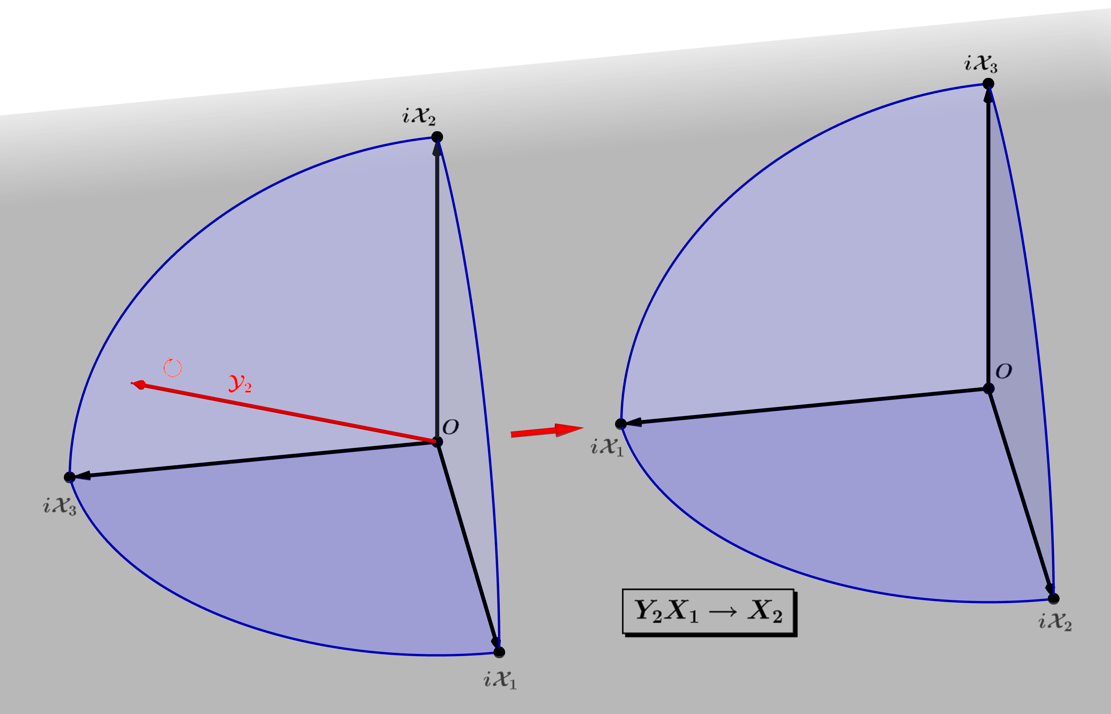
The second prod­uct Y2X1Y_{2}X_{1}, trans­forms the X1X_{1} al­ge­bra to the X2X_{2} al­ge­bra

Y2X1=X2→(010001100)(i0000i0i0)→(00i0i0i00),\begin{array}{r} Y_{2}X_{1} = X_{2} \rightarrow \begin{pmatrix} 0 & 1 & 0 \\ 0 & 0 & 1 \\ 1 & 0 & 0 \end{pmatrix}\begin{pmatrix} i & 0 & 0 \\ 0 & 0 & i \\ 0 & i & 0 \end{pmatrix} \rightarrow \begin{pmatrix} 0 & 0 & i \\ 0 & i & 0 \\ i & 0 & 0 \end{pmatrix}, \end{array}
(1.1.212)

where a cyclic modulo shift of all the el­e­ments in X1X_{1} has oc­curred by one entry to the left (Figure 1.1.23). The red Y2Y_{2} vector has a right cir­cu­lar arrow next to it, in­di­cat­ing the trans­for­ma­tion action it has on X1X_{1}, ro­tat­ing the X1X_{1} ver­tices in a clock­wise fash­ion around the axis of the Y2Y_{2} vector.

Figure
Figure 1.1.23 – The pro­jec­tive trans­for­ma­tion: Y2X1=X2∈S3ℂ/D3ℂY_{2}X_{1} = X_{2} \in S_{3\mathbb{C}}/D_{3\mathbb{C}}.

The third prod­uct, Y3X1Y_{3}X_{1}, trans­forms the X1X_{1} al­ge­bra in the op­pos­i­tive pro­jec­tive ori­en­ta­tion com­pared to the X3X_{3} al­ge­bra

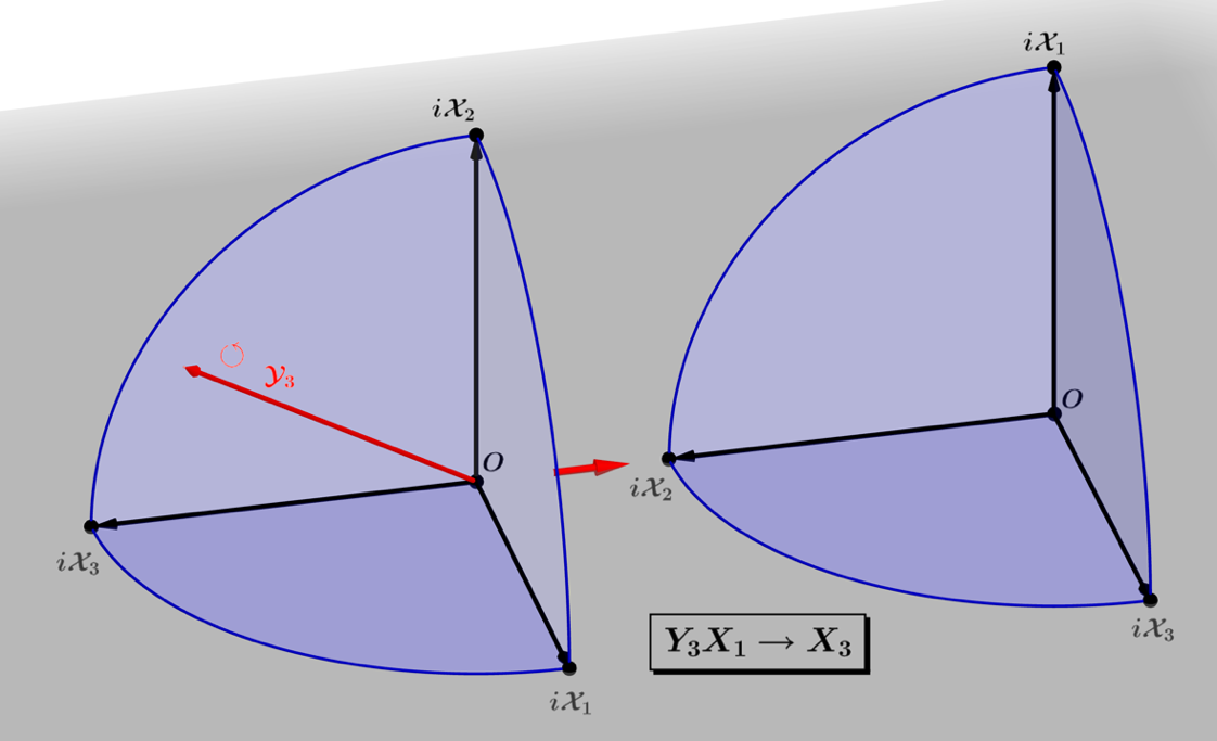
Y2X1=X3→(001100010)(i0000i0i0)→(0i0i0000i),\begin{array}{r} Y_{2}X_{1} = X_{3} \rightarrow \begin{pmatrix} 0 & 0 & 1 \\ 1 & 0 & 0 \\ 0 & 1 & 0 \end{pmatrix}\begin{pmatrix} i & 0 & 0 \\ 0 & 0 & i \\ 0 & i & 0 \end{pmatrix} \rightarrow \begin{pmatrix} 0 & i & 0 \\ i & 0 & 0 \\ 0 & 0 & i \end{pmatrix}, \end{array}
(1.1.213)

where a cyclic modulo shift of all the el­e­ments in X1X_{1} has oc­curred by one entry to the right (Figure 1.1.24). The red Y3Y_{3} vector with a left cir­cu­lar arrow next to it. Y3Y_{3} ro­tates the X1X_{1} ver­tices in a coun­ter­clock­wise manner about the Y3Y_{3} vector axis.

Figure
Figure 1.1.24 – The pro­jec­tive trans­for­ma­tion: Y3X1=X3∈S3ℂ/D3ℂY_{3}X_{1} = X_{3} \in S_{3\mathbb{C}}/D_{3\mathbb{C}}.

These ex­am­ples serve to un­der­stand better the geo­met­ric ro­ta­tions that result from the YjXkY_{j}X_{k} com­po­si­tion of func­tions. As ro­ta­tions, they occur in all three of the com­plex di­men­sions in the ℂ3\mathbb{C}^{3} space, dif­fer­ing from the more cus­tom­ary two-di­men­sion­al ro­ta­tions. The YjXkY_{j}X_{k} com­po­si­tions are not nec­es­sar­i­ly com­mu­ta­tive, with the ex­cep­tion of the iden­ti­ty, Y1Y_{1},

YjXk≠XkYj.\begin{array}{r} Y_{j}X_{k} \neq X_{k}Y_{j}. \end{array}
(1.1.214)

Using the al­ter­na­tive prod­uct orders for the pre­vi­ous ex­am­ples, we find

X1Y2=X3,  X1Y3=X2,\begin{array}{r} X_{1}Y_{2} = X_{3},\ \ X_{1}Y_{3} = X_{2}, \end{array}
(1.1.215)

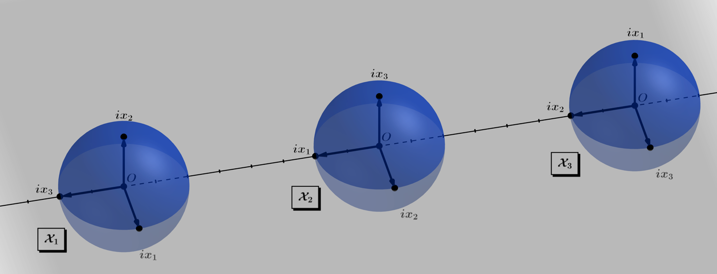
where these re­sults in­di­cate this change in prod­uct order has changed the di­rec­tion of ro­ta­tion for each. In the fol­low­ing figure, we con­sid­er the three pos­i­tive ori­en­ta­tions of the XjX_{j} al­ge­bras, which pro­ceed­ing from left to right are X1,X2,X3X_{1},X_{2},X_{3}, and the ixjix_{j} com­po­nents from the XjX_{j} al­ge­bras rep­re­sent ori­ent­ed vec­tors on the ℂ3\mathbb{C}^{3}-sphere.

Figure
Figure 1.1.25 – Pro­jec­tive ori­ent­ed XjX_{j} forms ∈S3ℂ/D3ℂ\in S_{3\mathbb{C}}/D_{3\mathbb{C}}.

The YjY_{j} al­ge­bras act to trans­form one XjX_{j} al­ge­bra to an­oth­er on the ℂ3\mathbb{C}^{3}-sphere, and we can rep­re­sent each YjY_{j} in sym­bol­ic form as

Y1=(ϵ),\begin{array}{r} Y_{1} = (\epsilon), \end{array}
(1.1.216)
Y2=(↺,↻),\begin{array}{r} Y_{2} = (\circlearrowleft,\circlearrowright), \end{array}
(1.1.217)
Y3=(↻,↺),\begin{array}{r} Y_{3} = (\circlearrowright,\circlearrowleft), \end{array}
(1.1.218)

where ϵ\epsilon sym­bol­izes the iden­ti­ty trans­for­ma­tion, and the left and right cir­cu­lar arrows for Y2,Y3Y_{2},Y_{3} in­di­cate the di­rec­tion of ro­ta­tion for the com­po­nent ver­tices about the YjY_{j} axis acting on XjX_{j}.

The geo­met­ric and ro­ta­tion­al spaces we per­ceive in space­time are con­tin­u­ous at the macro­scop­ic level, and many argue that spaces become pix­e­lat­ed at quan­tum dis­tances. Ro­ta­tions and boosts seem con­tin­u­ous at the macro­scop­ic level, un­der­scor­ing that these forms must have a math­e­mat­i­cal frame­work for pro­jec­tion to become con­tin­u­ous, or near-con­tin­u­ous, as geo­met­ric man­i­folds. The re­spon­si­ble frame­work is ex­po­nen­ti­a­tion, and for higher-di­men­sion­al Lie al­ge­bras, matrix ex­po­nen­ti­a­tion. The ex­po­nen­tial func­tion, it turns out, par­al­lels the in­te­gra­tion process, and we use their like­ness to con­sid­er how a form might project from a "zero-di­men­sion­al" point to man­i­fest in the form of a con­tin­u­ous man­i­fold. We

start by taking zero to rep­re­sent the "zero-di­men­sion­al" point, per­form­ing in­te­gra­tion in the X1X_{1}-space

∫0 dx1=𝒸,\begin{array}{r} \int_{}^{}0\ dx_{1}= \mathcal{c}, \end{array}
(1.1.219)

as­sum­ing a con­stant of in­te­gra­tion 𝒸\mathcal{c}. We take this con­stant 𝒸\mathcal{c} to be equal to unity, rep­re­sent­ing the value of a one-di­men­sion­al Lie al­ge­bra form, stem­ming from a volume in­te­gral of a "zero-di­men­sion­al" point. As the Lie al­ge­bra, let 𝒸\mathcal{c} be un­chang­ing and always equal to one

∀ 𝒸k=1.\begin{array}{r} \forall\ \mathcal{c}_{k} = 1. \end{array}
(1.1.220)

Con­tin­u­ing this process, while keep­ing to ∀ 𝒸k=1\forall\ \mathcal{c}_{k} = 1, we in­te­grate suc­ces­sive­ly six more times, find­ing the re­sult­ing par­tial series

∫x15120+x1424+x136+x122+x1+1 dx=x16720+x15120+x1424+x136+x122+x1+1.\begin{array}{r} \int_{}^{}{\frac{x_{1}^{5}}{120} + \frac{x_{1}^{4}}{24} + \frac{x_{1}^{3}}{6} + \frac{x_{1}^{2}}{2} + x_{1} + 1\ dx = \frac{x_{1}^{6}}{720} + \frac{x_{1}^{5}}{120} + \frac{x_{1}^{4}}{24} + \frac{x_{1}^{3}}{6} + \frac{x_{1}^{2}}{2} + x_{1} + 1.} \end{array}
(1.1.221)

In­te­grat­ing an in­fi­nite number of times will yield the ex­po­nen­tial series ex1e^{x_{1}}

∫…+x15120+x1424+x136+x122+x1+1 dx=ex1.\begin{array}{r} \int_{}^{}{\ldots + \frac{x_{1}^{5}}{120} + \frac{x_{1}^{4}}{24} + \frac{x_{1}^{3}}{6} + \frac{x_{1}^{2}}{2} + x_{1} + 1\ dx = e^{x_{1}}}. \end{array}
(1.1.222)

To define this math­e­mat­i­cal process, we in­tro­duce an in­te­gral like the kthk^{th} de­riv­a­tive no­ta­tion of a func­tion (∂n∂xn),\left( \frac{\partial^{n}}{\partial x^{n}} \right),as

D(x)−k[f(x)(𝒸k)],\begin{array}{r} D_{(x)}^{- k}\left\lbrack f(x)_{\left( \mathcal{c}_{k} \right)} \right\rbrack, \end{array}
(1.1.223)

which rep­re­sents the kthk^{th} in­te­gral of f(x)f(x) with re­spect to xx, with the con­tin­u­ous con­stant of in­te­gra­tion 𝒸k\mathcal{c}_{k}. As an ex­am­ple, for the in­te­gra­tion of zero from above, we can state math­e­mat­i­cal­ly that the fifth in­te­gral of 0 ∀ 𝒸k=1\forall\ \mathcal{c}_{k} = 1, is

D(x)−k[f(x)(𝒸k)]=1+x+x22!+x33!+x44!.\begin{array}{r} D_{(x)}^{- k}\left\lbrack f(x)_{\left( \mathcal{c}_{k} \right)} \right\rbrack = 1 + x + \frac{x^{2}}{2!} + \frac{x^{3}}{3!} + \frac{x^{4}}{4!}. \end{array}
(1.1.224)

De­f­i­n­i­tions (1.1.125-126) – For the vector 𝒸xj\mathcal{c}x_{j}, where xjx_{j} is a unit basis vector of some nn-di­men­sion­al vector space and 𝒸\mathcal{c} is a scalar con­stant,, the In­fi­nite In­te­gra­tion Func­tions fℝ−k(𝒸xj) , fℂ−k(𝒸ixj){\ f}_{\mathbb{R}}^{- k}\left( \mathcal{c}x_{j} \right)\ ,\ f_{\mathbb{C}}^{- k}\left( \mathcal{c}ix_{j} \right) start­ing at the zero point, for 𝒸xj∈ℝ, and 𝒸ixj∈ℂ\mathcal{c}x_{j}\in \mathbb{R},\ and\ \mathcal{c}ix_{j}\in \mathbb{C}, are de­fined as

fℝ−∞(𝒸xj)=limk→∞⁡(D(x)−k[xj(𝒸k)]) {∀ 𝒸∈ℝ ,∀ xj∈ℝn }=𝒸exj,\begin{array}{r} f_{\mathbb{R}}^{- \infty}\left( \mathcal{c}x_{j} \right) = \lim_{k \rightarrow \infty}\left( D_{(x)}^{- k}\left\lbrack {x_{j}}_{\left( \mathcal{c}_{k} \right)} \right\rbrack \right)\ \left\{ \forall\ \mathcal{c}\in \mathbb{R}\ ,\forall\ x_{j} \in \mathbb{R}^{n}\ \right\} = {\mathcal{c}e}^{x_{j}}, \end{array}
fℂ−∞(𝒸ixj)=limk→∞⁡(D(x)−k[ixj(𝒸k)]) {∀ 𝒸∈ℝ, ∀ ixj∈ℂn }=𝒸eixj.\begin{array}{r} f_{\mathbb{C}}^{- \infty}\left( \mathcal{c}ix_{j} \right) = \lim_{k \rightarrow \infty}\left( D_{(x)}^{- k}\left\lbrack {{ix}_{j}}{}_{\left( \mathcal{c}_{k} \right)} \right\rbrack \right)\ \left\{ \forall\ \mathcal{c}\in \mathbb{R},\ \forall\ {ix}_{j} \in \mathbb{C}^{n}\ \right\} = {\mathcal{c}e}^{ix_{j}}. \end{array}

The­o­rem (1.1.127) – Taking a unit basis vector xj,x_{j}, as a fixed form el­e­ment, the al­ge­bra func­tions fℝ(xj),fℂ(ixj)f_{\mathbb{R}}\left( x_{j} \right),f_{\mathbb{C}}\left( ix_{j} \right) are equal to the ex­po­nen­tial map­ping exp:𝔤→G∈ℝ,ℂexp:\mathfrak{g} \rightarrow G\in \mathbb{R},\mathbb{C} onto a con­tin­u­ous man­i­fold ∀ 𝔤=xj\forall\ \mathfrak{g} =x_{j}.

Proof –

∀ 𝔤={xj},   exp:𝔤→G=∑n=0∞(xj)nn!,\begin{array}{r} \forall\ \mathfrak{g} ={\{ x}_{j}\},\ \ \ exp:\mathfrak{g} \rightarrow G = \sum_{n = 0}^{\infty}\frac{\left( x_{j} \right)^{n}}{n!}, \end{array}
fℝ−k(xj)=…+xj5120+xj424+xj36+xj22+xj+1=∑n=0∞(xj)nn!=exp:𝔤→G ∀ 𝔤={xj},\begin{array}{r} f_{\mathbb{R}}^{- k}\left( x_{j} \right) = \ldots + \frac{x_{j}^{5}}{120} + \frac{x_{j}^{4}}{24} + \frac{x_{j}^{3}}{6} + \frac{x_{j}^{2}}{2} + x_{j} + 1 = \sum_{n = 0}^{\infty}\frac{\left( x_{j} \right)^{n}}{n!} = exp:\mathfrak{g} \rightarrow G\ \forall\ \mathfrak{g} ={\{ x}_{j}\}, \end{array}
fℂ−k(ixj)=…+(ixj)5120+(ixj)424+(ixj)36+(ixj)22+ixj+1=∑n=0∞(ixj)nn!=exp:𝔤→G ∀ 𝔤={ixj}.\begin{array}{r} f_{\mathbb{C}}^{- k}\left( ix_{j} \right) = \ldots + \frac{\left( ix_{j} \right)^{5}}{120} + \frac{\left( ix_{j} \right)^{4}}{24} + \frac{\left( ix_{j} \right)^{3}}{6} + \frac{\left( ix_{j} \right)^{2}}{2} + ix_{j} + 1 = \sum_{n = 0}^{\infty}\frac{\left( {ix}_{j} \right)^{n}}{n!} = exp:\mathfrak{g} \rightarrow G\ \forall\ \mathfrak{g} ={\{ ix}_{j}\}. \end{array}
□\square

We apply this to the two el­e­ments X3,Y3X_{3},Y_{3} from the S3ℂ/D3ℂS_{3\mathbb{C}}/D_{3\mathbb{C}} group, defin­ing scalar con­stants equal to 𝒸\mathcal{c}, where for X3X_{3}, we find

𝒸eiX3=…+𝒸(iX3)5120+𝒸(iX3)424+𝒸(iX3)36+𝒸(iX3)22+𝒸iX3+𝒸→\mathcal{c}e^{{iX}_{3}}= \ldots + \mathcal{c}\frac{\left( iX_{3} \right)^{5}}{120}+ \mathcal{c}\frac{\left( iX_{3} \right)^{4}}{24}+ \mathcal{c}\frac{\left( iX_{3} \right)^{3}}{6}+ \mathcal{c}\frac{\left( iX_{3} \right)^{2}}{2}+ \mathcal{c}iX_{3}+ \mathcal{c} \rightarrow
𝒸eX3=𝒸(…+(0ix350ix350000ix35)120+(x34000x34000x34)24+(0−ix330−ix330000−ix33)6+(−x32000−x32000−x32)2+(0ix30ix30000ix3)+(100010001))→\mathcal{c}e^{X_{3}}= \mathcal{c}\left( \begin{array}{r} \ldots + \frac{\begin{pmatrix} 0 & ix_{3}^{5} & 0 \\ ix_{3}^{5} & 0 & 0 \\ 0 & 0 & ix_{3}^{5} \end{pmatrix}}{120} + \frac{\begin{pmatrix} x_{3}^{4} & 0 & 0 \\ 0 & x_{3}^{4} & 0 \\ 0 & 0 & x_{3}^{4} \end{pmatrix}}{24} + \frac{\begin{pmatrix} 0 & - {ix}_{3}^{3} & 0 \\ - {ix}_{3}^{3} & 0 & 0 \\ 0 & 0 & - {ix}_{3}^{3} \end{pmatrix}}{6} + \\ \frac{\begin{pmatrix} - x_{3}^{2} & 0 & 0 \\ 0 & - x_{3}^{2} & 0 \\ 0 & 0 & - x_{3}^{2} \end{pmatrix}}{2} + \begin{pmatrix} 0 & ix_{3} & 0 \\ ix_{3} & 0 & 0 \\ 0 & 0 & ix_{3} \end{pmatrix} + \begin{pmatrix} 1 & 0 & 0 \\ 0 & 1 & 0 \\ 0 & 0 & 1 \end{pmatrix} \end{array} \right) \rightarrow
𝒸(1−x32+x34+…ix3−ix33+ix35+…0ix3−ix33+ix35+…1−x32+x34+…0001+ix3−x32−ix33+x34+ix35+…)\mathcal{c}\begin{pmatrix} 1{- x_{3}^{2} + x}_{3}^{4} + \ldots & ix_{3} - {ix}_{3}^{3} + ix_{3}^{5} + \ldots & 0 \\ ix_{3} - {ix}_{3}^{3} + ix_{3}^{5} + \ldots & {1 - x_{3}^{2} + x}_{3}^{4} + \ldots & 0 \\ 0 & 0 & 1 + {ix_{3} - x_{3}^{2} - {ix}_{3}^{3} + x}_{3}^{4} + ix_{3}^{5} + \ldots \end{pmatrix}
=𝒸(cos⁡(x3)isin(x3)0isin(x3)cos⁡(x3)000eix3),\begin{array}{r} = \mathcal{c}\begin{pmatrix} \cos\left( x_{3} \right) & isin\left( x_{3} \right) & 0 \\ isin\left( x_{3} \right) & \cos\left( x_{3} \right) & 0 \\ 0 & 0 & e^{ix_{3}} \end{pmatrix}, \end{array}
(1.1.228)

and for Y2Y_{2}

𝒸eY2=…+c(Y2)5120+c(Y2)424+c(Y2)36+c(Y2)22+cY2+c→\mathcal{c}e^{Y_{2}} = \ldots + c\frac{\left( Y_{2} \right)^{5}}{120} + c\frac{\left( Y_{2} \right)^{4}}{24} + c\frac{\left( Y_{2} \right)^{3}}{6} + c\frac{\left( Y_{2} \right)^{2}}{2} + cY_{2} + c \rightarrow
𝒸eY2=𝒸(1+y333!+y366!+…y322!+y355!+y388!+…y3+y344!+y377!+…y3+y344!+y377!+…1+y333!+y366!+…y322!+y355!+y388!+…y322!+y355!+y388!+…y3+y344!+y377!+…1+y333!+y366!+…).\begin{array}{r} \mathcal{c}e^{Y_{2}}= \mathcal{c}\begin{pmatrix} 1 + \frac{y_{3}^{3}}{3!} + \frac{y_{3}^{6}}{6!} + \ldots & \frac{y_{3}^{2}}{2!} + \frac{y_{3}^{5}}{5!} + \frac{y_{3}^{8}}{8!} + \ldots & y_{3} + \frac{y_{3}^{4}}{4!} + \frac{y_{3}^{7}}{7!} + \ldots \\ y_{3} + \frac{y_{3}^{4}}{4!} + \frac{y_{3}^{7}}{7!} + \ldots & 1 + \frac{y_{3}^{3}}{3!} + \frac{y_{3}^{6}}{6!} + \ldots & \frac{y_{3}^{2}}{2!} + \frac{y_{3}^{5}}{5!} + \frac{y_{3}^{8}}{8!} + \ldots \\ \frac{y_{3}^{2}}{2!} + \frac{y_{3}^{5}}{5!} + \frac{y_{3}^{8}}{8!} + \ldots & y_{3} + \frac{y_{3}^{4}}{4!} + \frac{y_{3}^{7}}{7!} + \ldots & 1 + \frac{y_{3}^{3}}{3!} + \frac{y_{3}^{6}}{6!} + \ldots \end{pmatrix}. \end{array}
(1.1.229)

The value for 𝒸\mathcal{c} re­lates to the mag­ni­tude of the ex­po­nen­tial series re­sult­ing from the in­te­gra­tion func­tions above. When 𝒸=1\mathcal{c} = 1, this fits the frame­work of a unit vector's ex­po­nen­tial map­ping. It is ap­pro­pri­ate to denote the com­bi­na­tion of mag­ni­tude and unit vector ori­en­ta­tion as 𝒸e1\mathcal{c}e_{1}, where e1e_{1} is the unit vector and 𝒸\mathcal{c} is a scalar mul­ti­ple, or mag­ni­tude, of this 𝒸e1\mathcal{c}e_{1} vector. The ex­po­nen­tial map­ping trans­forms the Lie al­ge­bra el­e­ments of a group from simple ro­ta­tions and re­flec­tions to in­fin­i­tes­i­mal trans­for­ma­tions on a con­tin­u­ous man­i­fold in ℂ3\mathbb{C}^{3} space. We have de­fined the in­fi­nite in­te­gra­tion func­tions fℝ−∞(𝒸xj)f_{\mathbb{R}}^{- \infty}\left( \mathcal{c}x_{j} \right) and fℂ−∞(𝒸ixj)f_{\mathbb{C}}^{- \infty}\left( \mathcal{c}ix_{j} \right), point­ing out the par­al­lel these have to the ex­po­nen­tial func­tion. The ori­ent­ed pro­jec­tion of a polyg­o­nal form through in­fi­nite in­te­gra­tion/ex­po­nen­ti­a­tion ex­tends that form into a con­tin­u­ous geo­met­ric space. These con­sid­er­a­tions are es­sen­tial in es­tab­lish­ing how some­thing out­side of a geo­met­ric space can give rise to the said space, in­ter­ject­ing the notion of causal­i­ty into our pro­ceed­ings.