In this section, mathematical curvature is considered and then applied in the context of mathematical physics. In particular, the hyperbolic asymptote serves as the boundary for the parametric curve , which approaches the asymptote per the limit
(1.3.256)
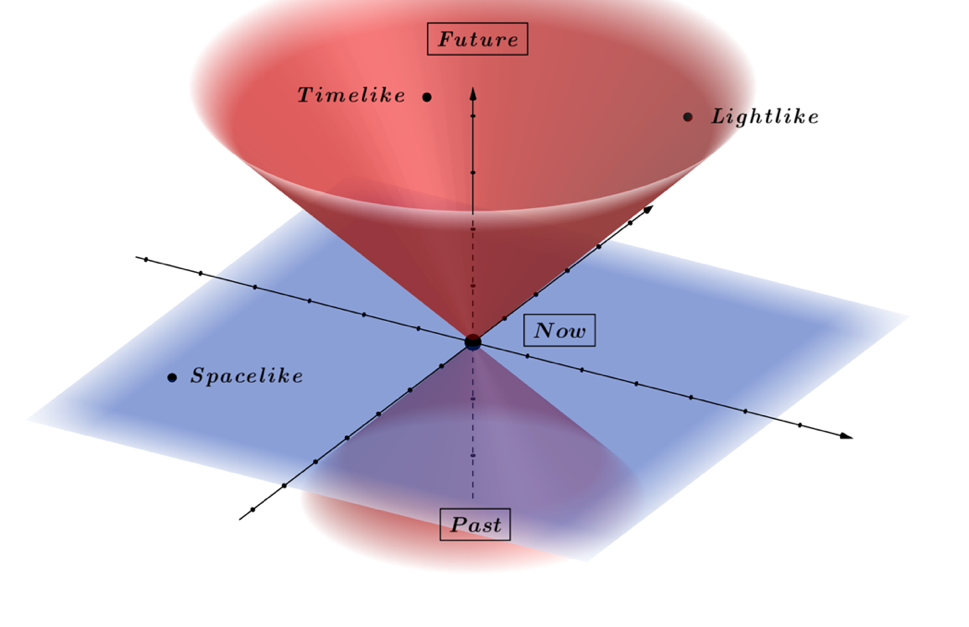
In physics, this asymptote is a boundary section of the relativistic light cone, which acts to separate time from space. The light cone is the basis for Einstein-Minkowski spacetime, which divides causality into a framework of the future and the past, relating to a temporal present. The light cone boundary sections the geometry into spacelike, timelike, and lightlike spaces. Figure 1.3.22 shows the time axis running from past to present and then to future. Space is depicted as the area outside the light cone, the time-space as in the cone, and the present/now as the center of the cone. We note that the spacelike region is situated on the horizontal plane passing by the origin, the lightlike is on the cone, and the time-like is in the volume space inside the lightcone. In section 1.1.26, we defined the dihedral group, whose basis revolves around an exceptional number, that being, which has multiple expressions, evidenced by the equivalent forms
(1.3.257)
It is also essential to consider that the negative forms also suffice for ,
(1.3.258)
and more precisely, is equal to
(1.3.259)
Figure 1.3.22 – The causal structure of the Einstein-Minkowski spacetime,
where the light cone separates past, present, future, and space.
Its counterpart, , can be stated in a similar way,
(1.3.260)
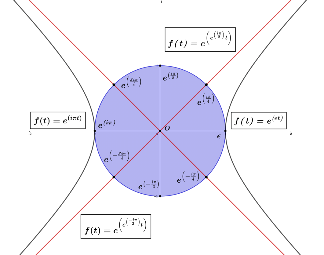
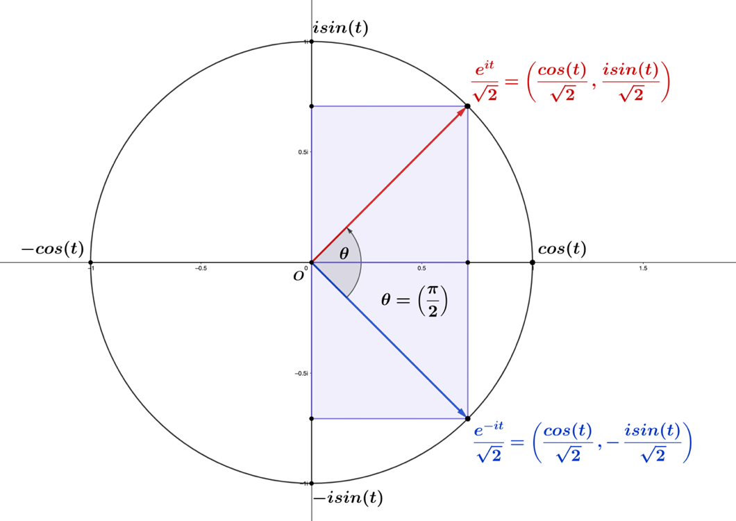
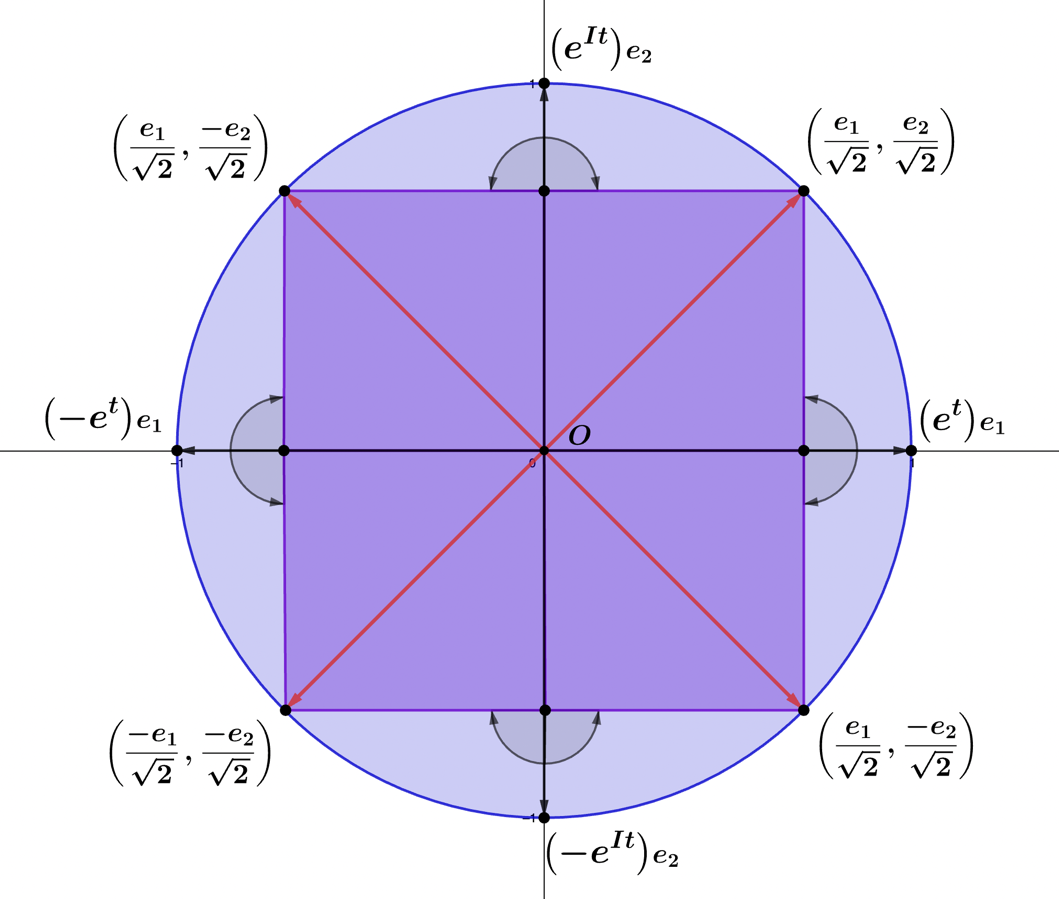
for which, all four of these numbers are located at points on the boundary of the complex unit circle through which the hyperbolic asymptotes emanate. Figure 1.3.23 represents how these numbers are oriented on the complex unit circle, demonstrated as the points where the red asymptotes meet the circle's boundary. The values that are boundary specific are depicted inside the complex unit circle, and the exponential mappings for the horizontally oriented unit hyperbola and circle are shown as the functions.
Figure 1.3.23 – The asymptotic numbers , and axis functions,
The asymptotes represent a balance between the sphere's positive curvature and the hyperbola's negative curvature. The question becomes, what functions serve as the asymptotes in complex space? We will use the implied complex geometry and the geometric product to find out. We start by taking the complex unit circle Lie group isomorphism,
(1.3.261)
and express this in vector format,
(1.3.262)
where the and functions represent variable-dependent scalar portions of the vector. Next, we define a vector, , to represent the asymptotic Lie algebra, , then consider the geometric product between the two vectors
(1.3.263)
By calculating the geometric product, we find the dot product equals
(1.3.264)
and the wedge product
(1.3.265)
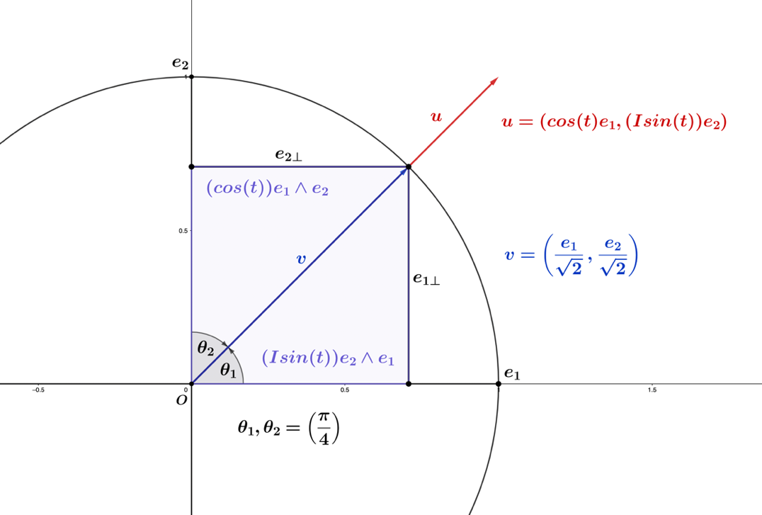
Figure 1.3.24 – The geometric product of the vectors and ,
By the isomorphism , the sum of the products representing is
(1.3.266)
a result of equal in magnitude contributions from the dot and wedge products. In Figure 1.3.24, the vectors that form this geometric product appear parallel. Despite this parallel appearance, incorporated is the nested bivector into the -vector, which acts to maintain a contribution from the wedge product in the result. Like the cosine and sine function example in the last section, we can distribute the bases containing the bivector , to represent the vector
(1.3.267)
which will result in the same geometric product once calculated. Next, we arrange the result into real and imaginary components, defining a two-dimensional parametric vector in the complex plane, as
(1.3.268)
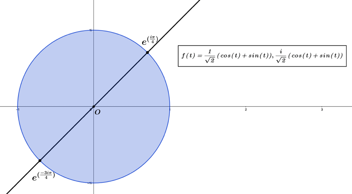
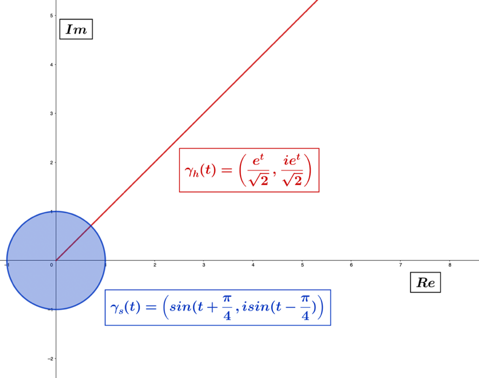
Figure 1.3.25 – The parametric equation in the complex plane.
The result is seen by plotting the function in Figure 1.3.25, revealing a flat and diagonally oriented curve consistent with the unit hyperbola's asymptote. This asymptotic consistency is appreciated given the flat curve intersects the complex unit circle at the points and The geometric intuition behind this example can be shown when we consider the complex plane, for functions oriented about the vertical axis, and for functions on the horizontal axis, as seen in Figure 1.3.26.
Figure 1.3.26 – Rotating the vector by radians in the complex trigonometric plane.
When rotating the vector in the complex plane by radians, it will align the vector functions. This is the same thing as adding the stationary vector , to the rotated vector , represented by the expression
(1.3.269)
which is the same result as the geometric product calculation. For , the complex conjugate of the function , is
(1.3.270)
and using the isomorphism, we set , for the , functions, and proceed to evaluate their geometric product
(1.3.271)
As these vectors are orthogonally related, we find the dot product equals zero
(1.3.272)
and the wedge product
(1.3.273)
where ultimately, the geometric product is solely due to the contribution from the wedge product
(1.3.274)
By way of the identity
(1.3.275)
we find that the geometric product produces a real-valued sine wave that is always , given that the in the expression shifts the waveform up by one on the vertical axis. To find the other asymptotic curve function, we reverse the vector order in the geometric product that yielded the function, to '
(1.3.276)
where we distributed the bivector, , in the bases of the original -vector, becoming, ,
(1.3.277)
The dot product calculates to
(1.3.278)
and the wedge product
(1.3.279)
leading to the result
(1.3.280)
After arranging it into a vector, we find is isomorphic to the complex conjugate form
(1.3.281)
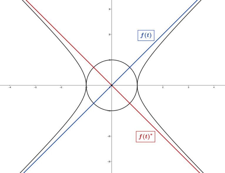
Figure 1.3.27 – Equations and represent the asymptotes of the unit hyperbola.
In Figure 1.3.27, we plot the functions in the complex plane with the unit hyperbola, where it can readily be seen these functions are the asymptote functions to the unit hyperbola. Given that
(1.3.282)
we can take the function to define the parametric function , and its complex conjugate , as follows
(1.3.283)
(1.3.284)
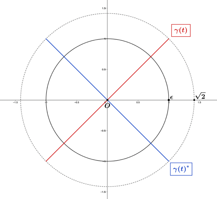
Figure 1.3.28 – The parametric plots and , extend to the circle of
radius,(dashed), for
In Figure 1.3.28, the functions and are plotted, revealing their flat curves extend beyond the unit circle to a maximum modulus equal to , for , occurring when equals
(1.3.285)
This extension beyond the unit circle boundary is due to the perpetual presence of equal magnitude real and imaginary values. This should be clear since the same trigonometric function represents the real and imaginary dimensions of We now define the time-based function , by using this compact form
(1.3.286)
which moves through time in the complex plane. The real portion of the wave function is the component, and the imaginary component is its orthogonally oriented counterpart.
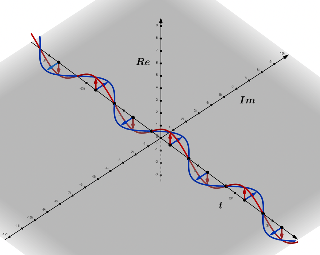
In Figure 1.3.29, we plot the function , which can be seen to move to the right in time, having orthogonally oriented wave components oscillating in the real and imaginary dimensions. The function has periodic roots in the time dimension, occurring when and wave components demonstrating peaks and troughs for . For the reader familiar with electromagnetic waves, these orthogonal waves are perfectly consistent with the characteristics of light. Also captured in the diagram is the intuition behind the wave-particle duality of light, meaning the phenomenology of light appears to be wave-like and particle-like. The particle-like characteristics of light manifest at each periodic root along the time dimension for , occurring twice per wave period as each wave component hits the time axis in unison. While the wave characteristic, inherent to its form, is defined by two orthogonally oriented waves oscillating through time.
Figure 1.3.29 - The wave function moving through time,
with orthogonally oriented waves oscillating in respective real and imaginary dimensions.
Electromagnetic waves also have spatial forms that travel through spatial distances in time, and we can define the complex plane wave with spatial and temporal components as follows
(1.3.287)
We then express , as the vector
(1.3.288)
and as before, the vector , is defined
(1.3.289)
We proceed to calculate the geometric product between the two vectors
(1.3.290)
finding the dot product portion equals
(1.3.291)
and the wedge product portion equals
(1.3.292)
leading to the following result for
(1.3.293)
which simplifies to the form
(1.3.294)
Using this result, we define the function to represent a wave traveling through the spatial and temporal dimensions, as
(1.3.295)
Maxwell's equations describe electromagnetism, and are defined by the following four equations in their differential forms:
(1.3.296)
(1.3.297)
(1.3.298)
(1.3.299)
where represents the electric field, and is the magnetic field. The first two equations are dot products, while the second two are cross-products. For the static equations, Gauss's law states that the electric flux passing through a closed surface is proportional to the total charge on its surface, and the magnetic flux passing through a closed surface is always equal to zero. While for the dynamic equations, Faraday's law states that a changing magnetic field in time produces a magnetic field, and Ampere's law says a changing electric field in time creates a magnetic field. The equations in free space without sources can be represented as
(1.3.300)
(1.3.301)
(1.3.302)
(1.3.303)
where and are now equal to zero.
Next, we define the and fields to be equal to the -wave function,
(1.3.304)
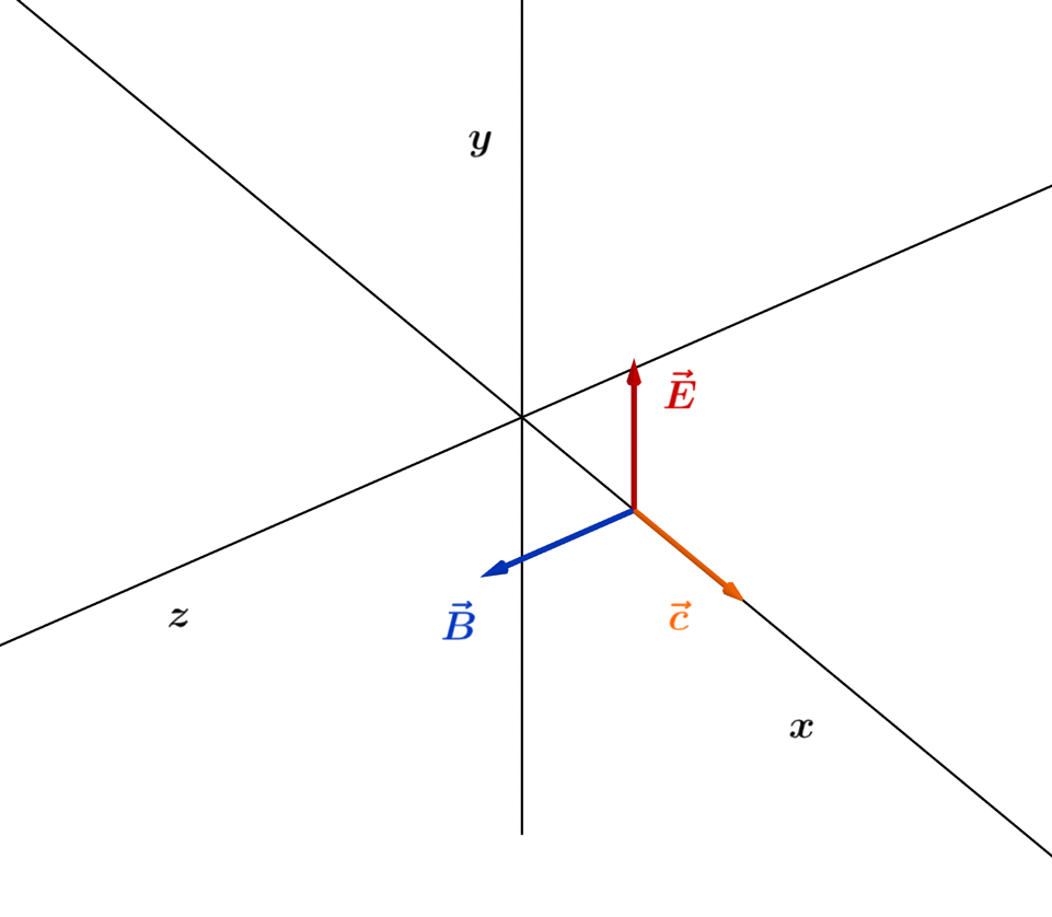
and consider a linearly polarized wave traveling at the speed of light in the -direction, with the electric field constrained to the direction, and the magnetic field constrained to the -direction (Figure 1.3.30).
Figure 1.3.30 – A linearly polarized plane wave is traveling at the speed of light along the -axis.
We set the following basis vectors for the three dimensions
(1.3.305)
which lend themselves to the following vector field representations
(1.3.306)
(1.3.307)
By evaluating the divergence for both fields
(1.3.308)
(1.3.309)
we find they equal zero, agreeing with Gauss' law and the magnetic law from the equations in free space. Next, we evaluate Faraday's law for our field functions, to find
(1.3.310)
noting the speed of light is equal to the following wavenumber-angular frequency relationship
(1.3.311)
The time derivative of the magnetic field is
(1.3.312)
and we equate the magnitudes of both sides of Faraday's law, and simplify
(1.3.313)
for which the differential equation holds. Next, we evaluate Ampere's law for our traveling wave
(1.3.314)
and the time derivative of the electric field
(1.3.315)
We equate the magnitudes of both sides of Ampere's law
(1.3.316)
to find this differential equation holds as well. The fact that the function is consistent with Maxwell's equations, shows that these asymptotic numbers and functions are light-based, specifically electromagnetic waves. The treatment of Maxwell's equations was cursory in this example, but we will return to this in more depth in the forthcoming volume concerning the dynamics of light.
The unified light functions are the final and arguably most impressive asymptotic light functions we consider in this section. The term unified, means that the spherical and hyperbolic geometries have been brought into alignment for the functions.
The defined vector
(1.3.317)
represents the -plane, for the , exponential functions oriented by their bases. We can rotate to any point on the function plane using the following geometric product,
(1.3.318)
where represents a point on the boundary of the unit circle in the -plane.
Figure 1.3.31 – Bivector Rotations
In Figure 1.3.31, we depict the -plane with hyperbolic and circular exponential functions oriented along the positive and negative ,-axes, adding red vectors to represent the axes of rotation for the -plane segments, using , as the rotation values. It turns out that rotating the -plane about these asymptotic axes, results in the light functions we are considering. By setting we transform the vector , as follows
(1.3.319)
for which, we have arranged the result by real and imaginary valued components. Real and imaginary hyperbolic and wave-like elements are noted in this result, which is readily seen in the complex plane by the parametric plot in Figure 1.3.32. The symmetric balance between the real and imaginary hyperbolic elements, results in a definitively flat geometry seen in the plot, while the wave elements comprise the unit circle geometry.
Figure 1.3.32 – Parametric plots of the hyperbolic and wave-like spherical elements of .
The vector is composed of scalar portions and bivectors portions, forming a function that is a hybridization of the unit hyperbola with the unit circle. We continue the process, rotating around the plane in a clockwise manner to all the asymptotic points and axes, by using the following products
(1.3.320)
(1.3.321)
(1.3.322)
(1.3.323)
(1.3.324)
(1.3.325)
(1.3.326)
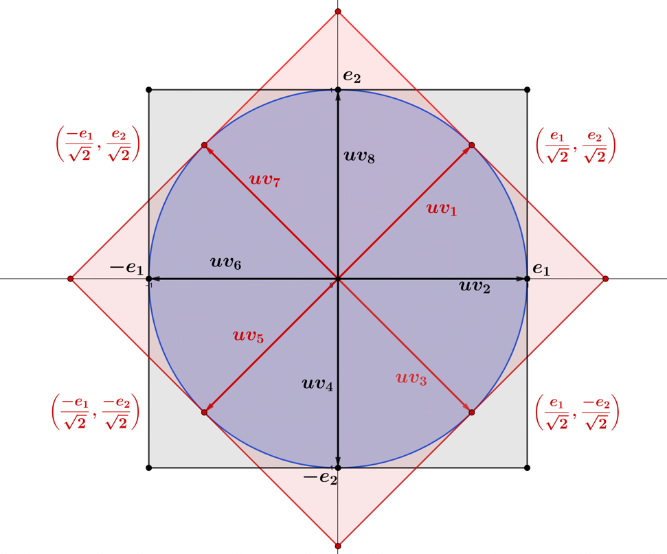
where we find results that are axis oriented for with even -values, and functions that are asymptote oriented for odd -values. The reader can orient themselves to the resulting vector arrangements by viewing Figure 1.3.33, from the perspective of the -plane, where the odd asymptotic vector functions are depicted in red, and the axis vector functions in black.
The square plane segments should stand out to the reader in Figure 1.3.33, whose significance is that the rotation of light occurs by moving oriented plane segments, which are the bivector forms of the geometric product. This differs from rotating a point or a vector in the complex two-dimensional plane, where the scalars and the bases are sufficient to describe the process. In the case of the asymptotic light functions, rotations occur in a higher-dimensional manifold, evidenced by the dynamics of bivector rotations.
Figure 1.3.33 – Oriented vectors and plane segments in the -plane.
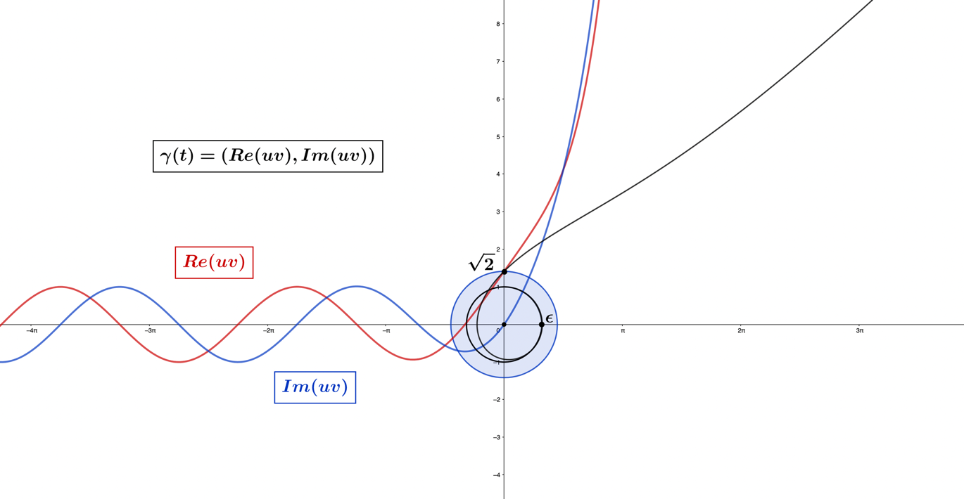
Next, we take a closer look at the light function by plotting in Figure 1.3.34, its imaginary and real components
(1.3.327)
(1.3.328)
which conveys that these light waveforms are a hybridization of wave and radial elements.
Figure 1.3.34 – Waveform plots: ,,
and the parametric plot,.
The circular trigonometric functions impart wave characteristics, while the hyperbolic functions impart radial extension. For , the exponential wave portion of each function dominates, while for , the exponential radius portion becomes omnipresent. This quality of the light functions clarifies what occurs when the macroscopy of classical physics becomes quantum physics at the microscopic level. Despite the dominance of the radial extension of the exponential function in the morphology to the right of the origin, the wave-like characteristics remain present in the form. On the other hand, to the left of the origin, it can also be said that despite the morphological wave dominance, the radial extension from the exponential function remains present, albeit in an attenuated form. The function plots show this as wave morphology dominance for , transforming to hyperbolic dominance for , after passing through in that process.
The -rotation vectors are not arbitrary, being all number forms related to , as mentioned at the onset of the section. The number is closely related to the vector What should not be overlooked is that the handedness of the geometric product can result in rotations in the opposite direction. So, the initial product evaluated was , with on the right side, which effectively rotates in the inverse direction of the related rotation , which is then effectively a rotation of by
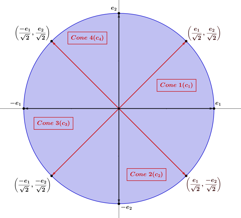
The functions form the asymptotic cones having the following matrix representations:
(1.3.329)
(1.3.330)
(1.3.331)
(1.3.332)
The top row of each cone matrix, denoted can take the parametric function form
(1.3.333)
and the bottom row, the form
(1.3.334)
The orientation of the cone segments can be seen in Figure 1.3.35, where the axes are the respective cone axes for The cone matrices all have determinants equal to zero, which occurs since the vector arrangement mimics the dot product. Using the first cone matrix as an example, we express the , vectors, as
(1.3.335)
Figure 1.3.35 – The asymptotic cone sections in the -plane.
We now calculate the dot product of the , vector components
(1.3.336)
where the result equals zero, and this is consistent with the two orthogonal vectors. The geometric product is therefore, equal to the wedge product
(1.3.337)
where the wedge product is equal to the vector squared. Now, we consider the vectors and , which represent the columns of the Cone 1 group
(1.3.338)
(1.3.339)
for which, the values for each vector represent the column vectors from the matrix. Next, we add the two vectors together
(1.3.340)
and the basis portions cancel, leading to a vector sum equal to the geometric product scaled by , orienting with the axis
(1.3.341)
It is easily verified that similar vector sums for the other cones hold. Obtained as follows:
(1.3.342)
(1.3.343)
(1.3.344)
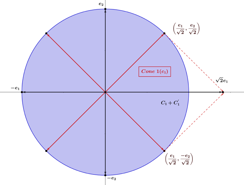
Geometrically, these sums represent the diagonals of the oriented parallelograms, formed by the pair of vectors. We demonstrate this for the case of the vector sum, in the figure below.
Figure 1.3.36 – The vector sum , represents
the diagonal of the oriented parallelogram formed by the vectors.
The importance of these vector addition results is that plays a central role in relativity and the perception of the speed of light. It will be considered in more detail toward the end of the book, but suffice it to say, represents the diagonal length of the complex unit square, which plays a significant role as the constant for the complex unit cube's shear transformations and maintains this invariant area representing the speed of light.
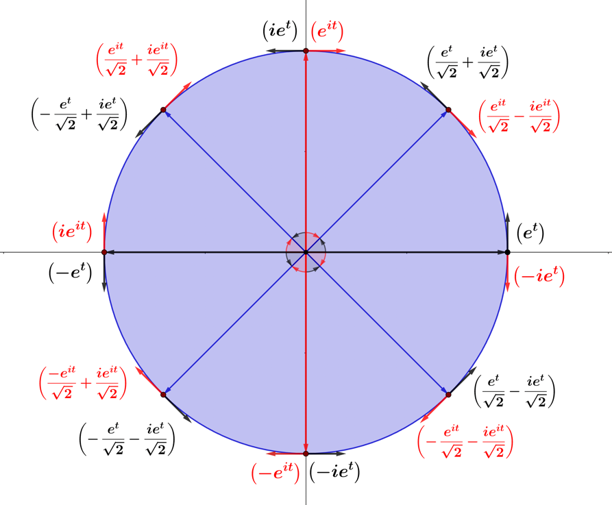
Figure 1.3.37 – Tangent vector map of the Light functions in the complex plane and angle space.
The light cones and light axes result from a dynamic process of circular and hyperbolic geometries moving past one another. These geometries should be considered out of phase in the complex angle space, which was alluded to earlier in the chapter and elucidated by the simple example , which holds for The light asymptotes have orthogonal relationships to the respective asymptotes oriented a distance away, as do the light axes. This phase difference, , defines the orthogonality in the complex plane for the light functions. The hyperbolic and circular planes can be viewed as rotating past one another in opposite directions. This is shown in Figure 1.3.37, where the chosen representation has the red tangent vectors of the circular geometry with negative/clockwise orientation, and the black tangent vectors of the hyperbolic geometry with positive/counterclockwise orientation. When the light functions are viewed in this manner, we can define the generalized unified light functions:
Definition (1.3.345) – The generalized spatial-temporal unified light functions,are defined, as
where the time-phased,, will be a multiple of the asymptotic angle,radians, the functions may also take on the spatial forms
Using the function, we set , and consider integer values for , starting at , then watch how the light system evolves
(1.3.346)
(1.3.347)
(1.3.348)
(1.3.349)
(1.3.350)
Apparent from the above, is the light system rotates in the clockwise direction with respect to the unified light function values for the asymptotes and axes. The representation of the light functions in Figure 1.3.37 is linked to the concept of torque in physics. Torque is typically defined as the magnitude of a tangential force component times the distance, implying the work done per unit angle. A torque vector is represented, as
(1.3.351)
for , the cross product between a position vector , originating at a point where torque is being measured to the point that a force is being applied, and a vector , representing the applied force. Given the presence of the cross product, it produces a vector that is orthogonal to both and , with an orientation that follows the right-hand rule. With the torque vector components described, torque can be defined, as
(1.3.352)
for , the angle between the force vector and the position vector . We can consider torque in terms of geometric algebra by considering the position vector in the parametric form,
(1.3.353)
for which, the unit bivector in the plane is the imaginary number , and noting the isomorphism , leading to the expression
(1.3.354)
In physics, the definition of work is the amount of energy transfer associated with the movement of an object over some distance, which is accomplished by an external force. For a system composed of a rotating body about a fixed axis, we can define the work done by a tangential force
(1.3.355)
The infinitesimal change in distance can be expressed in the radian measure , for , the radius vector, and , the infinitesimal displacement angle. We can rewrite the expression for work, as
(1.3.356)
for , the torque, resulting from the external and tangential force , leading to the identity
(1.3.357)
which can be solved for torque
(1.3.358)
In vector notation, the external force is expressed as , which has a tangential component force acting on a rotating body, assumed to be constant. We now state torque in terms of our vectors, as
(1.3.359)
where is the change of the vector over an infinitesimal displacement angle
(1.3.360)
This enables us to express torque using geometric algebra, as
(1.3.361)
and by expanding the position vector, we find
(1.3.362)
which we use to take the dot product with
(1.3.363)
In the above, we used the perpendicular basis vector in the force vector , to be consistent with the cross product's oriented normal vector. Notably, the result is consistent with the wedge product, given that
(1.3.364)
and this wedge product represents the torque of a system without and expressed as magnitudes per the traditional definition. This leads us to define the torque vector in geometric algebra notation, as
(1.3.365)
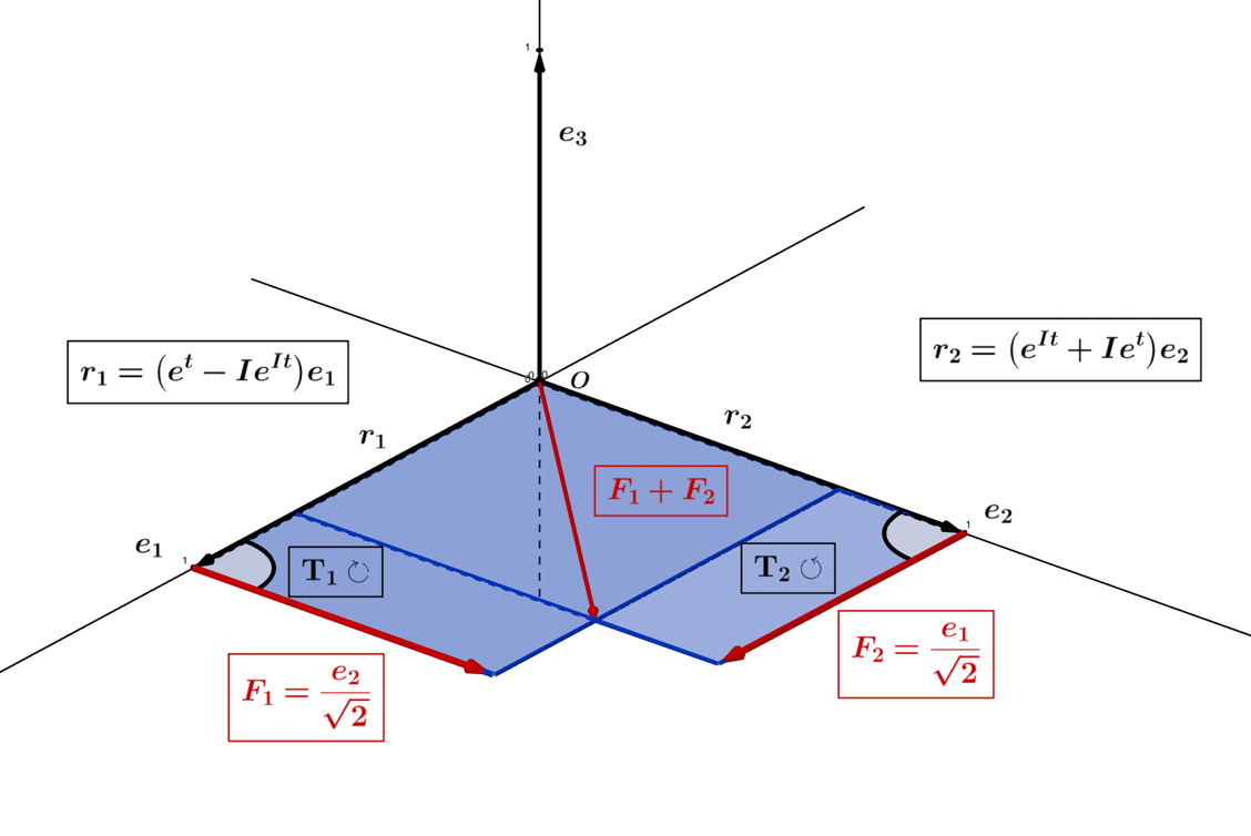
Using the bivectors native to geometric algebra, we do away with the need for a normal axis of rotation, which results from the cross-product. This turns out to be more consistent with the framework of the complex plane and its rotations, given that a normal axis to the plane of rotation is not mathematically required in the formalism. With torque defined in the context of geometric algebra, we apply it to the light functions described in this section. We consider the light system composed of two torques, by first, defining two position vectors
(1.3.366)
where we abstract that a position in the geometric space defines a time-dependent orientation of the complex unit circle and unit hyperbola, coinciding with the previously derived , geometric products. The applied forces on each of the position vectors are
(1.3.367)
having both magnitude and orientation. Next, we calculate the individual torque components
(1.3.368)
(1.3.369)
which are depicted in Figure 1.3.38, as the oriented bivectors , . These torque bivectors can be seen as equal in area but opposite in orientation.
Figure 1.3.38 – The geometric representation of the torques and .
The net torque of the function system is found by adding the torque components, which evaluate to
(1.3.370)
noting a result which is consistent with our previously derived, , geometric product.
So, the oriented torque bivector result depends on the function's distance in complex space, which varies by the value of the time variable . Intuitively, this should make sense, given that the -vector represents an oriented distance in the complex plane for which, a tangential force acts on the form associated with its vector head. Put in simple terms, is a torque function with results that orient in the complex plane. It should be noted, the ,, distance function vectors have a default torque that is particular to their forms, which stems from the presence of the complex unit circle in each. For instance, we take the portion from the torque calculation, to consider the form
(1.3.371)
in which, the simplification shows that is the orientation basis of the function. The exponential function does have an angular frequency, which is simply unitary , and setting , the oriented complex unit circle becomes
(1.3.372)
So, a torque occurs in the exponent of the function with an orthogonally oriented force, which is wedged with the unit radius basis vector . The exponent portion of the complex unit circle can now be seen in terms of its torque relationship, as
(1.3.373)
which amounts to a nested torque located in the exponent, representing work done over a distance in time, manifested as the radian distance in the tangent space. The exponential function has no angular rotation component, and therefore, does not have an innate torque like the complex unit circle. The reader should be aware that if we have -vectors, as follows
(1.3.374)
being the same absolute distance from the origin, when the same-valued forces are applied
(1.3.375)
the individual torque components are found to be
(1.3.376)
(1.3.377)
This leads to a net-torque force that is equal to zero, seen by evaluating the sum of torque components
(1.3.378)
So, we can think of a net-zero torque as the geometric product between two function vectors, oriented in an orthogonal basis in relation to one another. For two orthogonal function vectors , with a chosen orientation and the torque will be equivalent to the geometric product
(1.3.379)
If the net-torque
(1.3.380)
has rotation forces and , that are equal value, this leads to a wedge product equal to zero
(1.3.381)
given we are wedging a parallel scaled vector along its basis vector. By setting, , by associativity, we have the identity
(1.3.382)
Evaluating the geometric product , we find
(1.3.383)
where the dot product portion is zero, given that acts on perpendicularly, as does on By evaluating the net-torque , we find
(1.3.384)
which is equivalent to the geometric product of orthogonal vectors. We can further state by the defined orthogonal orientation of the vectors , that
(1.3.385)
which implies the geometric product equals
(1.3.386)
This primer on torque shows how it can be applied to the framework of the geometric product. Instead of being a scalar value, its meaning has been extended to that of a function oriented in the complex plane. We can mathematically conceptualize the forces acting on the circular and hyperbolic exponential functions in context to the unified light functions. To show this, we take the temporal unified light function as the example
(1.3.387)
where we have emphasized in bold, the portion in the exponents. This represents the forces acting on the function components ,, each serving to create torque in the complex functional plane. This is appreciated by defining the functional distance vector , as
(1.3.388)
and the force vector , is
(1.3.389)
Note, we have changed the sign of the exponent for , given the torque equation has the force on the right-hand side. Using the expression , we calculate the functional geometric torque
(1.3.390)
finding the force acts on the function , and acts on the function . We distribute the respective bivectors into the functions, finding that the net geometric torque equals
(1.3.391)
representing a sum of products, with the real force component matched to the -axis functional and the imaginary force component matched to the -axis functional. We set a preference to the -axis function , to denote the geometric torque as
(1.3.392)
and given that
(1.3.393)
is equivalent to
(1.3.394)
which represents the geometric algebra form of the unified light equations.
This section has served as our introduction to light's geometric and dynamical properties in the complex plane. The methods reflected here will soon be applied when we consider the higher-dimensional representations of form.