Masteries · Jason GlowneyArithmoí Book 1

Masteries

1.8.5 The Unit Invariant Mass and the Flowing Point Ideals

Pre­vi­ous­ly in the chap­ter, we con­sid­ered the ide­al­is­tic ex­am­ple of an in­vari­ant mass with zero ve­loc­i­ty in space, where the energy-mo­men­tum re­la­tion­ship of this system is re­duced to E=m0c2E = m_{0}c^{2}, by way of the fol­low­ing

E=m02c4+p2c2=m02c4+(m0v(0))2c2=m0c2.\begin{array}{r} E = \sqrt{m_{0}^{2}c^{4} + p^{2}c^{2}} = \sqrt{m_{0}^{2}c^{4} + \left( m_{0}v(0) \right)^{2}c^{2}} = m_{0}c^{2}. \end{array}
(1.8.209)

In spe­cial rel­a­tiv­i­ty and physics, an in­vari­ant mass is a quan­ti­ty that is the same for all ob­servers in all rest frames. Math­e­mat­i­cal­ly, an in­vari­ant mass re­sults from the point of in­ter­sec­tion be­tween spher­i­cal and hy­per­bol­ic geome­tries lo­cat­ed on the sin­gu­lar­i­ty's bound­ary. In the case of an in­vari­ant mass that is pur­port­ed to be in real space, the quan­ti­ty is static and not moving, im­ply­ing that the mass has no ki­net­ic energy. The tem­per­a­ture of a system is di­rect­ly re­lat­ed to the ki­net­ic energy of the ob­jects com­pos­ing it, and a system with zero ki­net­ic energy is, there­fore, a system at ab­solute zero in tem­per­a­ture.

Ab­solute zero is an ideal state when bound to space­time geom­e­try, given the in­fi­nite amount of work re­quired to cool the system to it. In physics, the Heisen­berg un­cer­tain­ty prin­ci­ple is the rea­son­ing behind the im­pos­si­bil­i­ty of ab­solute zero in space­time. By the prin­ci­ple in a system that ap­proach­es ab­solute zero, we are clos­ing in on a known pre­ci­sion for the mo­men­tum of its quan­tum par­ti­cles, which im­plies we are ap­proach­ing a com­plete lack in our abil­i­ty to know the po­si­tions of these quan­tum par­ti­cles. The Heisen­berg un­cer­tain­ty prin­ci­ple re­sults from the Fouri­er trans­form's math­e­mat­i­cal frame­work, where in­her­ent to its analy­sis, a func­tion and its Fouri­er trans­form cannot be lo­cal­ized in si­mul­tane­ity.

In space­time, zero ve­loc­i­ty and ab­solute zero are ideals. They do not exist, but math­e­mat­i­cal­ly, the ideals exist in Fouri­er trans­forms and the Uni­fied Field dy­nam­ics, where a trans­form can be lo­cal­ized en­tire­ly. At the same time, its func­tion is al­to­geth­er non-lo­cal­ized. A Lie al­ge­bra on the bound­ary of the in­fi­nite sphere of tan­gent spaces is wholly lo­cal­ized, while its matrix ex­po­nen­tial is in­fi­nite and non-lo­cal­ized. A gen­er­a­tor em­bod­ies the mo­men­tum frame­work, and the co­or­di­nate vec­tors it acts upon rep­re­sent the po­si­tions in the Uni­fied Field. The in­vari­ant mass with zero ve­loc­i­ty in space exists math­e­mat­i­cal­ly on the sin­gu­lar­i­ty's bound­ary, the bound­ary of the in­fi­nite sphere of tan­gent spaces.

To begin to con­sid­er the unit in­vari­ant mass, we first recall the hy­per­bol­ic Lorentz factor as it re­lates to energy-mo­men­tum

E=m0c2γ=m0c2cosh⁡(α),\begin{array}{r} E = m_{0}c^{2}\gamma = m_{0}c^{2}\cosh(\alpha), \end{array}
(1.8.210)

and solve this for the in­vari­ant mass

m0=Ec2γ=Ec2cosh⁡(α).\begin{array}{r} m_{0} = \frac{E}{c^{2}\gamma} = \frac{E}{c^{2}\cosh(\alpha)}. \end{array}
(1.8.211)

The in­ter­sec­tion be­tween spher­i­cal and hy­per­bol­ic geome­tries occurs at the point where the cosh⁡(α)\cosh(\alpha) func­tion has a joint so­lu­tion with the cos⁡(ω)\cos(\omega) func­tion, this being for α=0\alpha = 0 and ω=2πn\omega = 2\pi n, for ∈ℤ\in \mathbb{Z}, and we stay mind­ful of the equiv­a­lences for the fol­low­ing iden­ti­ties

e0=cosh⁡(0)=1,\begin{array}{r} e^{0} = \cosh(0) = 1, \end{array}
(1.8.212)
e2iπn=cos⁡(2iπn)=1.\begin{array}{r} e^{2i\pi n} = \cos(2i\pi n) = 1. \end{array}
(1.8.213)

In the con­text of the unit in­vari­ant mass, m0(ϵ),m_{0}(\epsilon),the common point of in­ter­sec­tion will be where the origin of the unit hy­per­bo­la meets the com­plex unit circle at the point 11 on the real-axis, and this point is also the iden­ti­ty, ϵ,\epsilon,for each.

In the two-di­men­sion­al space of ℂ\mathbb{C}, the al­ge­bra­ic uni­tary light so­lu­tion to c2=1c^{2} = 1 is the result of the prod­uct of the fol­low­ing light as­ymp­tote al­ge­bras

c2=e(iπ4)×e(−iπ4)=1,\begin{array}{r} c^{2} = e^{\left( \frac{i\pi}{4} \right)} \times e^{\left( - \frac{i\pi}{4} \right)} = 1, \end{array}
(1.8.214)

and is lo­cat­ed at the same iden­ti­ty point, ϵ\epsilon, on the sin­gu­lar­i­ty's bound­ary. Plug­ging these uni­tary values into our in­vari­ant mass ex­pres­sion, we have

m0(ϵ)=E(e(iπ4)×e(−iπ4))cosh⁡(0)=E1,\begin{array}{r} m_{0}(\epsilon) = \frac{E}{\left( e^{\left( \frac{i\pi}{4} \right)} \times e^{\left( - \frac{i\pi}{4} \right)} \right)\cosh(0)} = \frac{E}{1}, \end{array}
(1.8.215)

and this result rep­re­sents the co­a­les­cence of the as­ymp­tot­ic light al­ge­bras with that of the unit hy­per­bo­la's geom­e­try at the iden­ti­ty.

The co­a­les­cence point is on the sin­gu­lar­i­ty's bound­ary, and as such, we use the fol­low­ing ex­pres­sion for energy, EE,

E=ℏω,\begin{array}{r} E = \hslash\omega, \end{array}
(1.8.216)

where ℏ\hslash rep­re­sents the re­duced Planck's con­stant, and ω\omega the an­gu­lar fre­quen­cy.

The an­gu­lar fre­quen­cy in the energy ex­pres­sion for m0(ϵ)m_{0}(\epsilon), is the result of the so­lu­tion for eiω=ϵ,e^{i\omega} = \epsilon,oc­cur­ring at the iden­ti­ty when ω=2πn\omega = 2\pi n, which we sub­sti­tute into the energy ex­pres­sion

m0(ϵ)=ℏω1=ℏ(2πn)1, n∈ℤ\begin{array}{r} m_{0}(\epsilon) = \frac{\hslash\omega}{1} = \frac{\hslash(2\pi n)}{1},\ n\in \mathbb{Z} \end{array}
(1.8.217)

and given that

ℏ=h2π,\begin{array}{r} \hslash = \frac{h}{2\pi}, \end{array}
(1.8.218)

m0(ϵ)m_{0}(\epsilon) is equal to

m0(ϵ)=h1.\begin{array}{r} m_{0}(\epsilon) = \frac{h}{1}. \end{array}
(1.8.219)

Planck's con­stant, hh, is a fun­da­men­tal physics con­stant and, in SI units, is equal to the very small quan­ti­ty

h=6.62607015×10⁻³⁴J∙Hz−1,\begin{array}{r} h = 6.62607015 \times 10^{- 34}J \bullet Hz^{- 1}, \end{array}
(1.8.220)

in units of J∙Hz−1,J \bullet Hz^{- 1},rep­re­sent­ing SI units of energy over units of fre­quen­cy, equal to one cycle per second. The energy of a photon is de­fined as the prod­uct of Planck's con­stant with the photon's fre­quen­cy

E=hf,\begin{array}{r} E = hf, \end{array}
(1.8.221)

and the con­stant hh plays a fun­da­men­tal role in mass-energy equiv­a­lence, re­lat­ing fre­quen­cy and mass. The reader should note that the two energy ex­pres­sions are equiv­a­lent

E=hf=ℏω,\begin{array}{r} E = hf = \hslash\omega, \end{array}
(1.8.222)

ap­pre­ci­at­ed by the fact that ω=2πf\omega = 2\pi f, and for the m0(ϵ)m_{0}(\epsilon) case, we see that f=1f = 1, given ω=2π\omega = 2\pi. Geo­met­ri­cal­ly, Planck's con­stant is the radius of the unit sin­gu­lar­i­ty and, in the sense of on­to­log­i­cal math­e­mat­ics, is equal to unity. In clas­si­cal me­chan­ics, the energy ex­pres­sion hfhf is anal­o­gous to the energy/work con­cept of torque, where hh, Planck's con­stant, is the lever arm, and ff, the fre­quen­cy, is the force acting on it.

All the terms in the so­lu­tion to m0(ϵ)m_{0}(\epsilon), the unit in­vari­ant mass, are now joined at the co­a­les­cence point, the iden­ti­ty, which is the zero-di­men­sion­al point of pri­mor­dial light. The unit in­vari­ant mass rep­re­sents the math­e­mat­i­cal form the Uni­fied Field con­fers the mass char­ac­ter­is­tics upon and de­notes its small­est pos­si­ble value, ul­ti­mate­ly defin­ing the mass of the elec­tron and positron.

Figure
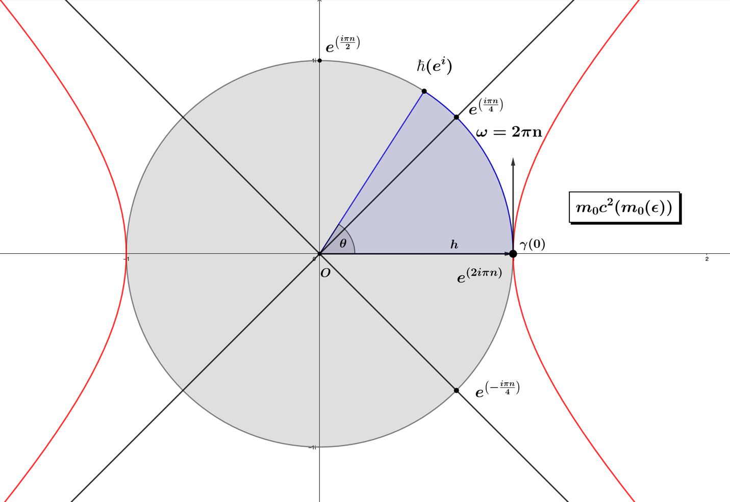
Figure 1.8.9 – The geom­e­try of the unit in­vari­ant mass in on­to­log­i­cal math­e­mat­ics. Com­plex unit circle in blue, the unit hy­per­bo­la in red, light as­ymp­totes in black, θ=iπn4\theta = \frac{i\pi n}{4}, Planck's h=1h = 1, re­duced Planck's ℏ=1(2π)\hslash = \frac{1}{(2\pi)}, and ω=2πn\omega = 2\pi n.

The figure above rep­re­sents the geo­met­ric co­a­les­cence and math­e­mat­i­cal basis for what the unit in­vari­ant mass, m0(ϵ)m_{0}(\epsilon), de­fines, which, like all as­pects of the Uni­fied Field, is a direct result of the split­ting of pri­mor­dial light of the zero-point, the iden­ti­ty. Every­thing out­lined re­gard­ing the unit in­vari­ant mass and its math­e­mat­i­cal un­der­pin­nings ap­plies to our higher-di­men­sion­al gen­er­a­tor forms. This is ap­pre­ci­at­ed by start­ing with the fol­low­ing matrix rep­re­sen­ta­tion of our gen­er­a­tor eA+iΩe^{\mathrm{A} + i\Omega}

eA+iΩ=γ(eiω(1+vc)000cos⁡(ω)+(vc)isin(ω)(vc)cos⁡(ω)+isin(ω)0(vc)cos⁡(ω)+isin(ω)cos⁡(ω)+(vc)isin(ω)),\begin{array}{r} e^{\mathrm{A} + i\Omega} = \gamma\begin{pmatrix} e^{i\omega}\left( 1 + \frac{v}{c} \right) & 0 & 0 \\ 0 & \cos{(\omega) + \left( \frac{v}{c} \right){isin}(\omega)} & \left( \frac{v}{c} \right)\cos(\omega) + {isin}(\omega) \\ 0 & \left( \frac{v}{c} \right)\cos(\omega) + {isin}(\omega) & \cos{(\omega) + \left( \frac{v}{c} \right){isin}(\omega)} \end{pmatrix}, \end{array}
(1.8.223)

which, after in­clud­ing our proper spher­i­cal/time and hy­per­bol­ic/space vari­ables, we can define as the ψ([A,Ω],[χ,τ])\psi\left( \lbrack \mathrm{A},\Omega\rbrack,\lbrack\chi,\tau\rbrack \right) wave­func­tion

ψ([A,Ω],[χ,τ])=γ(χ)(eiωτ(1+β)000cos⁡(ωτ)+βisin(ωτ)βcos⁡(ωτ)+isin(ωτ)0βcos⁡(ωτ)+isin(ωτ)cos⁡(ωτ)+βisin(ωτ)).\begin{array}{r} \psi\left( \lbrack \mathrm{A},\Omega\rbrack,\lbrack\chi,\tau\rbrack \right) = \gamma(\chi)\begin{pmatrix} e^{i\omega\tau}(1 + \beta) & 0 & 0 \\ 0 & \cos{(\omega\tau) + \beta{isin}(\omega\tau)} & \beta\cos(\omega\tau) + {isin}(\omega\tau) \\ 0 & \beta\cos(\omega\tau) + {isin}(\omega\tau) & \cos{(\omega\tau) + \beta{isin}(\omega\tau)} \end{pmatrix}. \end{array}
(1.8.224)

The uni­tary as­ymp­tot­ic light gen­er­a­tors we denote as 𝒸1\mathcal{c}_{1} and 𝒸7\mathcal{c}_{7}, which have the matrix rep­re­sen­ta­tions

𝒸1=(120000120120)+(i20000i20i20),\begin{array}{r} \mathcal{c}_{1} = \begin{pmatrix} \frac{1}{\sqrt{2}} & 0 & 0 \\ 0 & 0 & \frac{1}{\sqrt{2}} \\ 0 & \frac{1}{\sqrt{2}} & 0 \end{pmatrix} + \begin{pmatrix} \frac{i}{\sqrt{2}} & 0 & 0 \\ 0 & 0 & \frac{i}{\sqrt{2}} \\ 0 & \frac{i}{\sqrt{2}} & 0 \end{pmatrix}, \end{array}
(1.8.225)
𝒸7=(120000120120)−(i20000i20i20).\begin{array}{r} \mathcal{c}_{7} = \begin{pmatrix} \frac{1}{\sqrt{2}} & 0 & 0 \\ 0 & 0 & \frac{1}{\sqrt{2}} \\ 0 & \frac{1}{\sqrt{2}} & 0 \end{pmatrix} - \begin{pmatrix} \frac{i}{\sqrt{2}} & 0 & 0 \\ 0 & 0 & \frac{i}{\sqrt{2}} \\ 0 & \frac{i}{\sqrt{2}} & 0 \end{pmatrix}. \end{array}
(1.8.226)

We recall that the energy-mo­men­tum re­la­tion­ship is

E=m0c2γ,\begin{array}{r} \mathrm{E} = m_{0}c^{2}\gamma, \end{array}
(1.8.227)

and the geo­met­ric-de­pen­dent Schrödinger equa­tion de­rived in the last sec­tion is

−iℏψ([A,Ω],[χ,τ])∂τˆ=ℏ22mψ([A,Ω],[χ,τ])∂χ2ˆ,\begin{array}{r} - i\hslash\psi\left( \lbrack \mathrm{A},\Omega\rbrack,\lbrack\chi,\tau\rbrack \right)\widehat{\partial\tau} = \frac{\hslash^{2}}{2m}\psi\left( \lbrack \mathrm{A},\Omega\rbrack,\lbrack\chi,\tau\rbrack \right)\widehat{\partial\chi^{2}}, \end{array}
(1.8.228)

which we found to be equal to

ℏωψ([A,Ω],[χ,τ])=ℏ2α22m0ψ([A,Ω],[χ,τ]),\begin{array}{r} \hslash\omega\psi\left( \lbrack \mathrm{A},\Omega\rbrack,\lbrack\chi,\tau\rbrack \right) = \frac{\hslash^{2}\alpha^{2}}{2m_{0}}\psi\left( \lbrack \mathrm{A},\Omega\rbrack,\lbrack\chi,\tau\rbrack \right), \end{array}
(1.8.229)

where the α2\alpha^{2} term rep­re­sents the wavenum­ber squared, k2k^{2}. From the right-hand side of the equa­tion above, we take the ex­pres­sion that mul­ti­plies the wave­func­tion, ℏ2α22m0,\frac{\hslash^{2}\alpha^{2}}{2m_{0}},and given that, for matter waves, the wavenum­ber is equal to

k=pℏ=2mEℏ,\begin{array}{r} k = \frac{p}{\hslash} = \frac{\sqrt{2mE}}{\hslash}, \end{array}
(1.8.230)

we can ex­press it as the fol­low­ing mo­men­tum re­la­tion­ship

ℏ2α22m0=ℏ22m0(pℏ)2.\begin{array}{r} \frac{\hslash^{2}\alpha^{2}}{2m_{0}} = \frac{\hslash^{2}}{2m_{0}}\left( \frac{p}{\hslash} \right)^{2}. \end{array}
(1.8.231)

In the above, the ℏ2\hslash^{2} terms cancel, and after sub­sti­tut­ing p=2m0Ep = \sqrt{2m_{0}E}, the ex­pres­sion be­comes

ℏ2α22m0=p22m0=(2m0E)22m0.\begin{array}{r} \frac{\hslash^{2}\alpha^{2}}{2m_{0}} = \frac{p^{2}}{2m_{0}} = \frac{\left( \sqrt{2m_{0}E} \right)^{2}}{2m_{0}}. \end{array}
(1.8.232)

We use the matter wave energy equiv­a­lence E=m0c2E = m_{0}c^{2}, and cancel the like terms to find

ℏ2α22m0=(2m0(m0c2))22m0=m0c2,\begin{array}{r} \frac{\hslash^{2}\alpha^{2}}{2m_{0}} = \frac{\left( \sqrt{2m_{0}\left( m_{0}c^{2} \right)} \right)^{2}}{2m_{0}} = m_{0}c^{2}, \end{array}
(1.8.233)

where we have ar­rived at the m0c2m_{0}c^{2} from the energy-mo­men­tum re­la­tion E=m0c2γ\mathrm{E} = m_{0}c^{2}\gamma, and the geo­met­ric-de­pen­dent Schrödinger equa­tion is found to equal

ℏωψ([A,Ω],[χ,τ])=m0c2ψ([A,Ω],[χ,τ]).\begin{array}{r} \hslash\omega\psi\left( \lbrack \mathrm{A},\Omega\rbrack,\lbrack\chi,\tau\rbrack \right) = m_{0}c^{2}\psi\left( \lbrack \mathrm{A},\Omega\rbrack,\lbrack\chi,\tau\rbrack \right). \end{array}
(1.8.234)

Using the wave func­tion form

ψ([A,Ω],[χ,τ])=γ(χ)(eiωτ(1+β)000cos⁡(ωτ)+βisin(ωτ)βcos⁡(ωτ)+isin(ωτ)0βcos⁡(ωτ)+isin(ωτ)cos⁡(ωτ)+βisin(ωτ)),\begin{array}{r} \psi\left( \lbrack \mathrm{A},\Omega\rbrack,\lbrack\chi,\tau\rbrack \right) = \gamma(\chi)\begin{pmatrix} e^{i\omega\tau}(1 + \beta) & 0 & 0 \\ 0 & \cos{(\omega\tau) + \beta{isin}(\omega\tau)} & \beta\cos(\omega\tau) + {isin}(\omega\tau) \\ 0 & \beta\cos(\omega\tau) + {isin}(\omega\tau) & \cos{(\omega\tau) + \beta{isin}(\omega\tau)} \end{pmatrix}, \end{array}
(1.8.235)

E=m0c2γ\mathrm{E} = m_{0}c^{2}\gamma can be ex­pressed using the geo­met­ric-de­pen­dent Schrödinger equa­tion as

ℏωψ([A,Ω],[χ,τ])=m0(𝒸1∙𝒸7)γ(χ)(eiωτ(1+β)000cos⁡(ωτ)+βisin(ωτ)βcos⁡(ωτ)+isin(ωτ)0βcos⁡(ωτ)+isin(ωτ)cos⁡(ωτ)+βisin(ωτ)),\begin{array}{r} \hslash\omega\psi\left( \lbrack \mathrm{A},\Omega\rbrack,\lbrack\chi,\tau\rbrack \right) = m_{0}\left( \mathcal{c}_{1} \bullet \mathcal{c}_{7} \right)\gamma(\chi)\begin{pmatrix} e^{i\omega\tau}(1 + \beta) & 0 & 0 \\ 0 & \cos{(\omega\tau) + \beta{isin}(\omega\tau)} & \beta\cos(\omega\tau) + {isin}(\omega\tau) \\ 0 & \beta\cos(\omega\tau) + {isin}(\omega\tau) & \cos{(\omega\tau) + \beta{isin}(\omega\tau)} \end{pmatrix}, \end{array}
(1.8.236)

where c2=𝒸1∙𝒸7c^{2} = \mathcal{c}_{1} \bullet \mathcal{c}_{7} rep­re­sents the prod­uct of the light as­ymp­totes. The m0(𝒸1∙𝒸7)m_{0}\left( \mathcal{c}_{1} \bullet \mathcal{c}_{7} \right) on the right-hand side, when ex­pand­ed in matrix form, is

m0(𝒸1∙𝒸7)=m0((120000120120)+(i20000i20i20))((120000120120)−(i20000i20i20)),\begin{array}{r} m_{0}\left( \mathcal{c}_{1} \bullet \mathcal{c}_{7} \right) = m_{0}\left( \begin{pmatrix} \frac{1}{\sqrt{2}} & 0 & 0 \\ 0 & 0 & \frac{1}{\sqrt{2}} \\ 0 & \frac{1}{\sqrt{2}} & 0 \end{pmatrix} + \begin{pmatrix} \frac{i}{\sqrt{2}} & 0 & 0 \\ 0 & 0 & \frac{i}{\sqrt{2}} \\ 0 & \frac{i}{\sqrt{2}} & 0 \end{pmatrix} \right)\left( \begin{pmatrix} \frac{1}{\sqrt{2}} & 0 & 0 \\ 0 & 0 & \frac{1}{\sqrt{2}} \\ 0 & \frac{1}{\sqrt{2}} & 0 \end{pmatrix} - \begin{pmatrix} \frac{i}{\sqrt{2}} & 0 & 0 \\ 0 & 0 & \frac{i}{\sqrt{2}} \\ 0 & \frac{i}{\sqrt{2}} & 0 \end{pmatrix} \right), \end{array}
(1.8.237)

which simply equals

m0(𝒸1∙𝒸7)=m0(100010001),\begin{array}{r} m_{0}\left( \mathcal{c}_{1} \bullet \mathcal{c}_{7} \right) = m_{0}\begin{pmatrix} 1 & 0 & 0 \\ 0 & 1 & 0 \\ 0 & 0 & 1 \end{pmatrix}, \end{array}
(1.8.238)

and given that γ(χ)=cosh⁡(αχ)\gamma(\chi) = \cosh(\alpha\chi), the right-hand side in its en­tire­ty, m0c2ψ([A,Ω],[χ,τ]),m_{0}c^{2}\psi\left( \lbrack \mathrm{A},\Omega\rbrack,\lbrack\chi,\tau\rbrack \right),is equal to

m0(cosh⁡(αχ)000cosh⁡(αχ)000cosh⁡(αχ))(eiωτ(1+β)000cos⁡(ωτ)+βisin(ωτ)βcos⁡(ωτ)+isin(ωτ)0βcos⁡(ωτ)+isin(ωτ)cos⁡(ωτ)+βisin(ωτ)).\begin{array}{r} m_{0}\begin{pmatrix} \cosh(\alpha\chi) & 0 & 0 \\ 0 & \cosh(\alpha\chi) & 0 \\ 0 & 0 & \cosh(\alpha\chi) \end{pmatrix}\begin{pmatrix} e^{i\omega\tau}(1 + \beta) & 0 & 0 \\ 0 & \cos{(\omega\tau) + \beta{isin}(\omega\tau)} & \beta\cos(\omega\tau) + {isin}(\omega\tau) \\ 0 & \beta\cos(\omega\tau) + {isin}(\omega\tau) & \cos{(\omega\tau) + \beta{isin}(\omega\tau)} \end{pmatrix}. \end{array}
(1.8.239)

For the right-hand side, we set the proper hy­per­bol­ic/space value to one, χ=1\chi = 1, and sub­sti­tute the same values for our vari­ables, α=0\alpha = 0, ω=2π\omega = 2\pi. Given that βγ=sinh⁡(α)\beta\gamma = \sinh(\alpha), when α=0\alpha = 0, βγ=0\beta\gamma = 0, and the right-hand side sim­pli­fies to

m0c2ψ([A,Ω],[χ,τ])=m0(100010001)(100010001)=(m0000m0000m0).\begin{array}{r} m_{0}c^{2}\psi\left( \lbrack \mathrm{A},\Omega\rbrack,\lbrack\chi,\tau\rbrack \right) = m_{0}\begin{pmatrix} 1 & 0 & 0 \\ 0 & 1 & 0 \\ 0 & 0 & 1 \end{pmatrix}\begin{pmatrix} 1 & 0 & 0 \\ 0 & 1 & 0 \\ 0 & 0 & 1 \end{pmatrix} = \begin{pmatrix} m_{0} & 0 & 0 \\ 0 & m_{0} & 0 \\ 0 & 0 & m_{0} \end{pmatrix}. \end{array}
(1.8.240)

For the left-hand side, we sub­sti­tute ℏ=12π\hslash = \frac{1}{2\pi} and once again χ=1,α=0\chi = 1,\alpha = 0, ω=2π\omega = 2\pi, to find it sim­pli­fies to the iden­ti­ty matrix

ℏωψ([A,Ω],[χ,τ])=(12π)2π(100010001)=ϵ,\begin{array}{r} \hslash\omega\psi\left( \lbrack \mathrm{A},\Omega\rbrack,\lbrack\chi,\tau\rbrack \right) = \left( \frac{1}{2\pi} \right)2\pi\begin{pmatrix} 1 & 0 & 0 \\ 0 & 1 & 0 \\ 0 & 0 & 1 \end{pmatrix} = \epsilon, \end{array}
(1.8.241)

and the so­lu­tion to the geo­met­ric-de­pen­dent Schrödinger equa­tion with our uni­tary choice of vari­ables

ℏωψ([A,Ω],[χ,τ])=m0c2ψ([A,Ω],[χ,τ]),\begin{array}{r} \hslash\omega\psi\left( \lbrack \mathrm{A},\Omega\rbrack,\lbrack\chi,\tau\rbrack \right) = m_{0}c^{2}\psi\left( \lbrack \mathrm{A},\Omega\rbrack,\lbrack\chi,\tau\rbrack \right), \end{array}
(1.8.242)

is equal to

(100010001)=(m0000m0000m0),\begin{array}{r} \begin{pmatrix} 1 & 0 & 0 \\ 0 & 1 & 0 \\ 0 & 0 & 1 \end{pmatrix} = \begin{pmatrix} m_{0} & 0 & 0 \\ 0 & m_{0} & 0 \\ 0 & 0 & m_{0} \end{pmatrix}, \end{array}
(1.8.243)

rep­re­sent­ing the unit in­vari­ant mass m0=ϵ.m_{0} = \epsilon.