Masteries · Jason GlowneyArithmoí Book 1

Masteries

1.7.5 Discussion and Summary

The prime-count­ing func­tion π(n)\pi(n) de­fines the number of primes oc­cur­ring for ≤n∈ℕ\leq n\in \mathbb{N} and the prime number the­o­rem states that π(n)\pi(n) is as­ymp­tot­ic to nn over the log­a­rithm of nn

π(n)∼nln⁡(n), n∈ℕ,\begin{array}{r} \pi(n)\sim\frac{n}{\ln(n)},\ n\in \mathbb{N}, \end{array}
(1.7.396)

which, as an es­ti­mate, is at­trib­ut­able to Gauss and Le­gendre. The prime number the­o­rem states that the ratio π(n)\pi(n) to nln⁡(n)\frac{n}{\ln(n)} ap­proach­es 11 as nn ap­proach­es in­fin­i­ty

limn→∞⁡(π(n)(nln⁡(n)))=1,\begin{array}{r} \lim_{n \rightarrow \infty}\left( \frac{\pi(n)}{\left( \frac{n}{\ln(n)} \right)} \right) = 1, \end{array}
(1.7.397)

and that the prime num­bers are as­ymp­tot­ic in their dis­tri­b­u­tion, be­com­ing less fre­quent in ap­pear­ance for larger num­bers. The prob­a­bil­i­ty that a chosen nat­ur­al number nn is prime is ap­prox­i­mate­ly

n∈ℙ≈1ln⁡(n).\begin{array}{r} n\in \mathbb{P} \approx\frac{1}{\ln(n)}. \end{array}
(1.7.398)
Figure
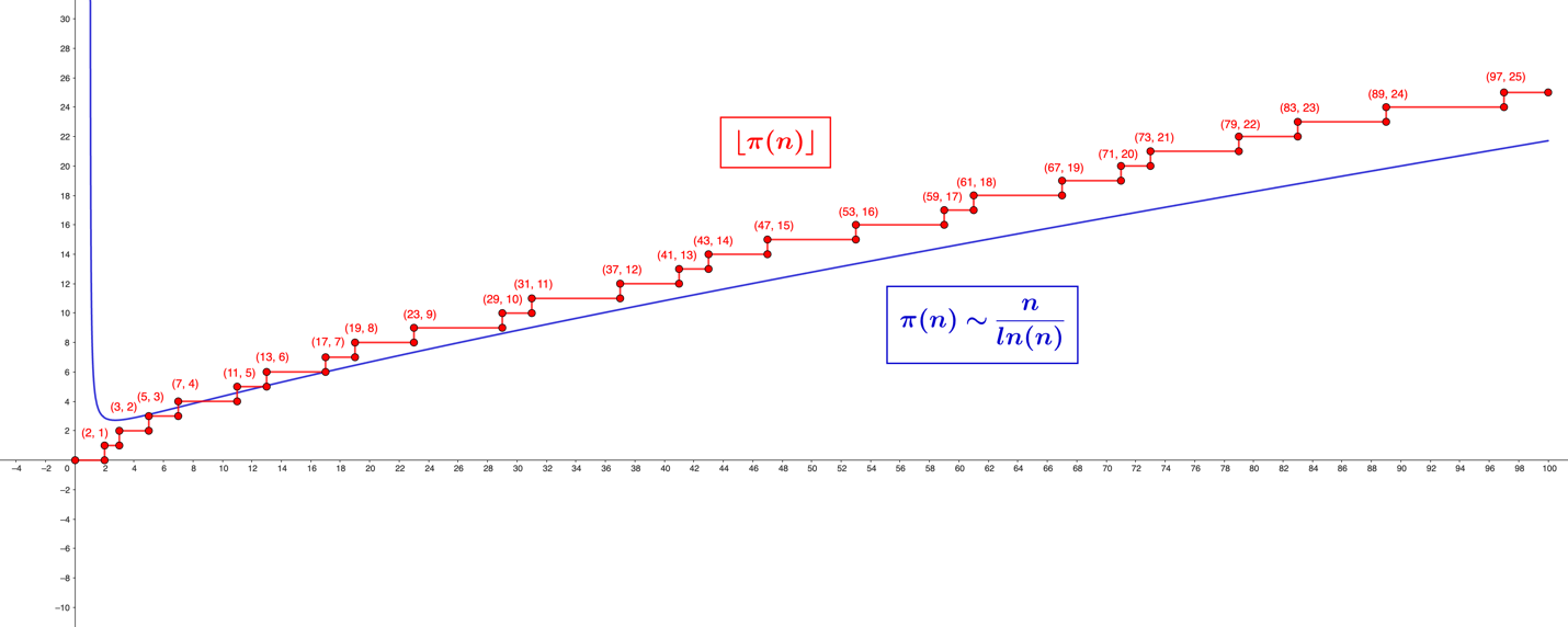
Figure 1.7.40 – The Prime-Count­ing Func­tion π(n)=⌊ π(n)⌋\pi(n) = \left\lfloor \left. \ \pi(n) \right\rfloor \right.and π(n)∼nln⁡(n)\pi(n)\sim\frac{n}{\ln(n)} for the first 25 primes (n=[1,100]).\left( n = \lbrack 1,100\rbrack \right).

In Figure 1.7.40, the prime-count­ing func­tion π(n)\pi(n) is rep­re­sent­ed as the floor func­tion ⌊ π(n)⌋\left\lfloor \left. \ \pi(n) \right\rfloor \right., which is com­pared with the rec­i­p­ro­cal log­a­rithm ap­prox­i­ma­tion π(n)∼nln⁡(n)\pi(n)\sim\frac{n}{\ln(n)}. A better es­ti­mate re­lates the prime-count­ing func­tion to the offset log­a­rith­mic in­te­gral

π(n)∼Li(n)=∫2n1ln⁡(t) dt,\begin{array}{r} \pi(n)\sim Li(n) = \int_{2}^{n}{\frac{1}{\ln(t)}\ dt}, \end{array}
(1.7.399)

which yields small­er and small­er rel­a­tive errors for in­creas­ing nn.

In 1859, Bernard Rie­mann1 used an­a­lyt­ic con­tin­u­a­tion to extend the study of har­mon­ic series from real to com­plex vari­ables and fur­ther to es­tab­lish the re­la­tion­ship be­tween the zeta zeroes and the dis­tri­b­u­tion of the primes. In the form of a series, the zeta func­tion is de­fined as

ζ(s)=∑n=1∞1ns=11s+12s+13s+…,   s∈ℂ,\begin{array}{r} \zeta(s) = \sum_{n = 1}^{\infty}{\frac{1}{n^{s}} = \frac{1}{1^{s}} + \frac{1}{2^{s}} + \frac{1}{3^{s}} + \ldots},\ \ \ s\in \mathbb{C}, \end{array}
(1.7.400)

for the com­plex vari­able s∈ℂs\in \mathbb{C}. Like the Euler prod­uct over the reals, ζ(s)\zeta(s) has the prime number equiv­a­lence

ζ(s)=∏p prime11−p−s=11−2−s×11−3−s×11−5−s×11−7−s×11−11−s×…,   s∈ℂ.\begin{array}{r} \zeta(s) = \prod_{p\ prime}^{}{\frac{1}{1 - p^{- s}} = \frac{1}{1 - 2^{- s}} \times \frac{1}{1 - 3^{- s}} \times \frac{1}{1 - 5^{- s}} \times \frac{1}{1 - 7^{- s}} \times \frac{1}{1 - 11^{- s}} \times \ldots,\ \ \ s\in \mathbb{C}}. \end{array}
(1.7.401)

For Re(s)>1Re(s) > 1, we can rep­re­sent the Rie­mann zeta func­tion as the con­ver­gent in­te­gral

ζ(s)=1Γ(s)∫0∞xs−1ex−1dx,\begin{array}{r} \zeta(s) = \frac{1}{\Gamma(s)}\int_{0}^{\infty}{\frac{x^{s - 1}}{e^{x} - 1}dx}, \end{array}
(1.7.402)

in which the gamma func­tion Γ(s)\Gamma(s) is also con­ver­gent

Γ(s)=∫0∞xs−1e−xdx,\begin{array}{r} \Gamma(s) = \int_{0}^{\infty}{x^{s - 1}e^{- x}}dx, \end{array}
(1.7.403)

and when s∈ℤ+s \in \mathbb{Z}^{+}, the gamma func­tion is re­lat­ed to the fac­to­r­i­al func­tion by

Γ(s)=(s−1)!.\begin{array}{r} \Gamma(s) = (s - 1)!. \end{array}
(1.7.404)

The an­a­lyt­ic con­tin­u­a­tion begins with the re­la­tion­ship be­tween the ζ(s)\zeta(s) func­tion and the Dirich­let eta func­tion η(s)\eta(s)

(1−22s)ζ(s)=η(s)=∑n=1∞(−1)n+1ns=11s−12s+13s−…,   s∈ℂ,\begin{array}{r} \left( 1 - \frac{2}{2^{s}} \right)\zeta(s) = \eta(s) = \sum_{n = 1}^{\infty}\frac{( - 1)^{n + 1}}{n^{s}} = \frac{1}{1^{s}} - \frac{1}{2^{s}} + \frac{1}{3^{s}} - \ldots,\ \ \ s\in \mathbb{C}, \end{array}
(1.7.405)

for which the con­ver­gence of the zeta func­tion on the right-hand side ex­tends to all Re(s)>0Re(s) > 0, except for (1−22s)=0\left( 1 - \frac{2}{2^{s}} \right) = 0, oc­cur­ring when n∈ℤn\in \mathbb{Z} in the fol­low­ing ex­pres­sion for ss

s=1+2iπnln⁡(2).\begin{array}{r} s = 1 + \frac{2i\pi n}{\ln(2)}. \end{array}
(1.7.406)

The con­ver­gence issues for these zeros can be solved using the limit ap­proach. By the re­la­tion­ship with the η(s)\eta(s) func­tion, the zeta func­tion can be de­fined as

ζ(s)=η(s)(1−22s),   s∈ℂ.\begin{array}{r} \zeta(s) = \frac{\eta(s)}{\left( 1 - \frac{2}{2^{s}} \right)},\ \ \ s\in \mathbb{C}. \end{array}
(1.7.407)

The in­fa­mous Rie­mann Hy­poth­e­sis con­cerns the zeros out­side the region of con­ver­gence for the in­fi­nite series stated in Eq. (1.7.400). Rie­mann showed the an­a­lyt­ic con­tin­u­a­tion of the ζ(s)\zeta(s) func­tion sat­is­fies the func­tion­al equa­tion

ζ(s)=2sπs−1sin⁡(πs2)Γ(1−s)ζ(1−s),\begin{array}{r} \zeta(s) = 2^{s}\pi^{s - 1}\sin\left( \frac{\pi s}{2} \right)\Gamma(1 - s)\zeta(1 - s), \end{array}
(1.7.408)

in which the triv­ial zeros man­i­fest when ss equals a neg­a­tive even in­te­ger value. The non-triv­ial zeros all lie in what is de­fined as the crit­i­cal strip be­tween real values of 00 and 11. Rie­mann fur­ther hy­poth­e­sizes that all the non-triv­ial zeros have a real por­tion ss equal to one-half, Re(s)=12Re(s) = \frac{1}{2}, laying on the crit­i­cal line.

In the chap­ter, we extend the nat­ur­al num­bers to the com­plex domain, taking the form of cyclic groups GnG_{n}, with prime number groups GpG_{p} being fur­ther clas­si­fied as simple groups. The reader has likely gath­ered that the min­i­mal el­e­ment, ini­tial­ly pre­sent­ed in Sec­tion 1.4.5, is syn­ony­mous with a group's pri­ma­ry gen­er­a­tor(s), ca­pa­ble of self-prod­ucts that yield all el­e­ments of the de­fined group, ⟨gk⟩=G\left\langle g^{k} \right\rangle = G. For n>1∈ℕn > 1 \in \mathbb{N}, a pos­i­tive and neg­a­tive ori­ent­ed pri­ma­ry gen­er­a­tor are guar­an­teed to exist, noting in the case for n=2n = 2, these two pri­ma­ry gen­er­a­tors are su­per­im­posed on the com­plex unit circle

⟨g2+⟩=e2iπ[12]=⟨g2−⟩=e2iπ[−12]=−1.\begin{array}{r} \left\langle g_{2}^{+} \right\rangle = e^{2i\pi\left\lbrack \frac{1}{2} \right\rbrack} = \left\langle g_{2}^{-} \right\rangle = e^{2i\pi\left\lbrack - \frac{1}{2} \right\rbrack} = - 1. \end{array}
(1.7.409)

When con­sid­ered in the com­plex domain and as groups, the law of net-zero can easily be ap­plied to the prime num­bers. The most straight­for­ward is the con­ju­gate re­la­tion­ship that exists be­tween any pri­ma­ry gen­er­a­tors ⟨gn+⟩\left\langle g_{n}^{+} \right\rangle, ⟨gn−⟩\left\langle g_{n}^{-} \right\rangle, which form the prod­uct

⟨gn+⟩∙⟨gn−⟩=e2iπ[1n]∙e2iπ[−1n]=1.\begin{array}{r} \left\langle g_{n}^{+} \right\rangle \bullet \left\langle g_{n}^{-} \right\rangle = e^{2i\pi\left\lbrack \frac{1}{n} \right\rbrack} \bullet e^{2i\pi\left\lbrack - \frac{1}{n} \right\rbrack} = 1. \end{array}
(1.7.410)

For the pos­i­tive and ex­tend­ing wave­form func­tions g+(ℤ+(n))g^{+}\left( \mathbb{Z}^{+}(n) \right) and g−(ℤ+(n))g^{-}\left( \mathbb{Z}^{+}(n) \right), de­pict­ed in Fig­ures 1.7.37-39, their net-zero coun­ter­parts are in­verse­ly re­lat­ed in both their spher­i­cal and spa­tial ar­gu­ments. This is seen using the ex­am­ple of the prime number n=7n = 7, with

g+(ℤ+(7))=e(2iπ[17]+ln⁡(7))=7e(2iπ[17]),\begin{array}{r} g^{+}\left( \mathbb{Z}^{+}(7) \right) = e^{\left( 2i\pi\left\lbrack \frac{1}{7} \right\rbrack + \ln(7) \right)} = {7e}^{\left( 2i\pi\left\lbrack \frac{1}{7} \right\rbrack \right)}, \end{array}
(1.7.411)
g−(ℤ+(7))=e(2iπ[−17]+ln⁡(7))=7e(2iπ[−17]),\begin{array}{r} g^{-}\left( \mathbb{Z}^{+}(7) \right) = e^{\left( 2i\pi\left\lbrack - \frac{1}{7} \right\rbrack + \ln(7) \right)} = {7e}^{\left( 2i\pi\left\lbrack - \frac{1}{7} \right\rbrack \right)}, \end{array}
(1.7.412)

which have the cor­re­spond­ing in­vers­es

g−(ℤ−+(7))=e(2iπ[17]−ln⁡(7))=e2iπ[−17]7,\begin{array}{r} g^{-}\left( \mathbb{Z}_{-}^{+}(7) \right) = e^{\left( 2i\pi\left\lbrack \frac{1}{7} \right\rbrack - \ln(7) \right)} = \frac{e^{2i\pi\left\lbrack - \frac{1}{7} \right\rbrack}}{7}, \end{array}
(1.7.413)
g+(ℤ−+(7))=e(2iπ[−17]−ln⁡(7))=e2iπ[17]7.\begin{array}{r} g^{+}\left( \mathbb{Z}_{-}^{+}(7) \right) = e^{\left( 2i\pi\left\lbrack - \frac{1}{7} \right\rbrack - \ln(7) \right)} = \frac{e^{2i\pi\left\lbrack \frac{1}{7} \right\rbrack}}{7}. \end{array}
(1.7.414)

The para­met­ric func­tions defin­ing the con­tract­ing rec­i­p­ro­cal wave­forms are

g+(t)=(cos⁡(2πt)t−1,isin(2πt)t−1),   t∈ℝ,\begin{array}{r} g^{+}(t) = \left( \cos\left( \frac{2\pi}{t} \right)t^{- 1},isin\left( \frac{2\pi}{t} \right)t^{- 1} \right),\ \ \ t\in \mathbb{R}, \end{array}
(1.7.415)
g−(t)=(cos⁡(2πt)t−1,−isin(2πt)t−1),   t∈ℝ,\begin{array}{r} g^{-}(t) = \left( \cos\left( \frac{2\pi}{t} \right)t^{- 1}, - isin\left( \frac{2\pi}{t} \right)t^{- 1} \right),\ \ \ t\in \mathbb{R}, \end{array}
(1.7.416)

and are plot­ted in Figure 1.7.41. The con­tract­ing rec­i­p­ro­cal nat­ur­al number para­met­ric equa­tions are for the values of n∈tn \in t, for n∈ℕn\in \mathbb{N}

g+(n)=(cos⁡(2πn)n−1,isin(2πn)n−1),   n∈ℕ,\begin{array}{r} g^{+}(n) = \left( \cos\left( \frac{2\pi}{n} \right)n^{- 1},isin\left( \frac{2\pi}{n} \right)n^{- 1} \right),\ \ \ n\in \mathbb{N}, \end{array}
(1.7.417)
g−(n)=(cos⁡(2πn)n−1,−isin(2πn)n−1),   n∈ℕ.\begin{array}{r} g^{-}(n) = \left( \cos\left( \frac{2\pi}{n} \right)n^{- 1}, - isin\left( \frac{2\pi}{n} \right)n^{- 1} \right),\ \ \ n\in \mathbb{N}. \end{array}
(1.7.418)
Figure
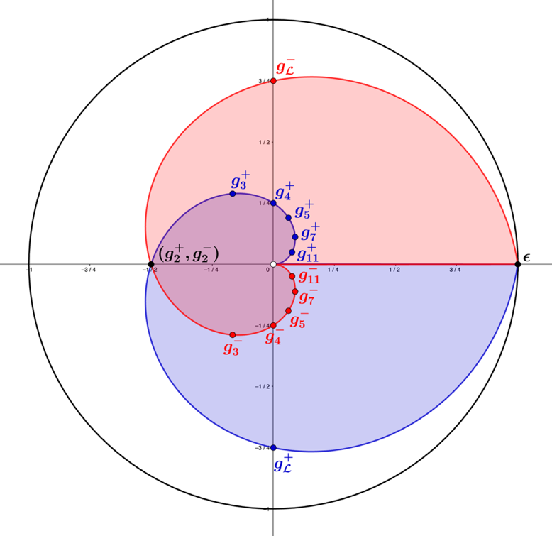
Figure 1.7.41 – The cyclic group rep­re­sen­ta­tions of the nat­ur­al num­bers n∈tn \in t pro­ject­ed

onto the unit disc for the rec­i­p­ro­cal time func­tion f(t)=1t, t∈ℝf(t) = \frac{1}{t},\ t\in \mathbb{R}.

The g+(t),g−(t)g^{+}(t),g^{-}(t) curves in­ter­sect the real-axis at the iden­ti­ty ϵ\epsilon and g2+,g2−g_{2}^{+},g_{2}^{-}, and in­ter­sect the imag­i­nary-axis at g4+,g4−g_{4}^{+},g_{4}^{-}, and the non-in­te­ger values gℒ−,gℒ+g_{\mathcal{L}}^{-},g_{\mathcal{L}}^{+}, for t=43t = \frac{4}{3}. The sub­script ℒ\mathcal{L} in­di­cates that these are light num­bers, ev­i­denced by the values of these points on each curve

gℒ−=143e2iπ[− 143]=34eiπ2,\begin{array}{r} g_{\mathcal{L}}^{-} = \frac{1}{\frac{4}{3}}e^{2i\pi\left\lbrack - \ \frac{1}{\frac{4}{3}} \right\rbrack} = \frac{3}{4}e^{\frac{i\pi}{2}}, \end{array}
(1.7.419)
gℒ+=143e2iπ[143]=34e−iπ2.\begin{array}{r} g_{\mathcal{L}}^{+} = \frac{1}{\frac{4}{3}}e^{2i\pi\left\lbrack \frac{1}{\frac{4}{3}} \right\rbrack} = \frac{3}{4}e^{- \frac{i\pi}{2}}. \end{array}
(1.7.420)

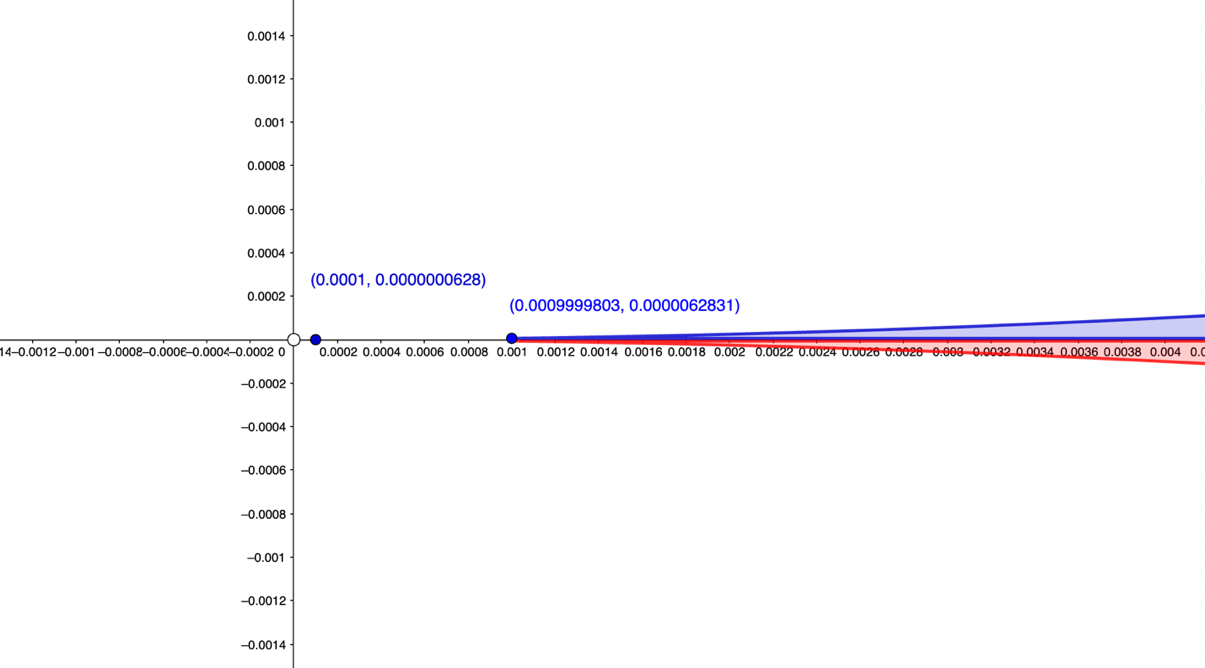
Two car­dioids in Figure 1.7.41 are formed by the in­ter­sec­tion of the para­met­ric func­tion g+(t),g−(t)g^{+}(t),g^{-}(t). The larger one is formed over the in­ter­val t=[1,12]t = \left\lbrack 1,\frac{1}{2} \right\rbrack for g+(t),g−(t)g^{+}(t),g^{-}(t), be­com­ing a closed curve when t≥12t \geq \frac{1}{2}. The small­er car­dioid only ap­proach­es a close curve as t→∞t \rightarrow \infty. This is ap­pre­ci­at­ed by zoom­ing into the origin for the plot on the in­ter­val t=[1,1000]t = \lbrack 1,1000\rbrack, where blue points on the g+(t)g^{+}(t) para­met­ric curve are plot­ted for t=1000t = 1000 and t=10,000t = 10,000.

Figure
Figure 1.7.42- The second car­dioid ap­proach­es closed form as t→∞t \rightarrow \infty.

The rec­i­p­ro­cal func­tions are re­lat­ed to log­a­rith­mic spi­rals and the log­a­rithm func­tion itself, seen by con­sid­er­ing that the in­te­grals of the fol­low­ing form are equal to ln⁡(n)\ln(n)

∫1n1t|cos⁡(2πt)|2+|isin(2πt)|2dt=ln⁡(n).\begin{array}{r} \int_{1}^{n}{\frac{1}{t}\sqrt{\left| \cos\left( \frac{2\pi}{t} \right) \right|^{2} + \left| isin\left( \frac{2\pi}{t} \right) \right|^{2}}}dt = \ln(n). \end{array}
(1.7.421)

As dis­cussed, many number theory func­tions and series are re­lat­ed to the study of prime num­bers, in­clud­ing the fac­to­r­i­al and the ex­tend­ed gamma func­tions, the digam­ma func­tion, the har­mon­ic series, the log­a­rithm func­tion, and the Euler-Mascheroni con­stant. The Rie­mann zeta func­tion ex­tends the har­mon­ic series by rais­ing the el­e­ments of the series to com­plex powers of ss. The chap­ter aimed to see nat­ur­al num­bers ∈ℤ\in \mathbb{Z}, the in­te­gers ∈ℝ\in \mathbb{R}, and the real num­bers ∈ℂ\in \mathbb{C}. All on­to­log­i­cal num­bers are in­ter­re­lat­ed, and groups are num­bers in motion. When seen in this frame­work, all the prime num­bers are present in the sin­gu­lar­i­ty. Num­bers and their amal­gams as group rep­re­sen­ta­tions can extend beyond the ini­tial sin­gu­lar state's uni­tary bound­ary, made pos­si­ble by their co­in­ci­dent in­verse form that con­tracts.

Are prime num­bers valid on­to­log­i­cal­ly, mean­ing they have rel­e­vance to the nature of being? Or are they just math­e­mat­ics fan­fare? Prime num­bers play an es­sen­tial role in cryp­tog­ra­phy, but this falls short of the de­f­i­n­i­tion of being on­to­log­i­cal­ly sig­nif­i­cant.

In 1972, Hugh Mont­gomery2 shared recent find­ings re­lat­ed to his work on the zeros of the Rie­mann zeta func­tion with Atle Sel­berg, a pro­fes­sor at Prince­ton's In­sti­tute for Ad­vanced Study. Mont­gomery had found the dis­tri­b­u­tion of the zeros on the crit­i­cal line of ζ(s)\zeta(s) tended to repel be­tween the neigh­bor­ing levels. Mont­gomery would also share what is now called the pair cor­re­la­tion con­jec­ture with Free­man Dyson, whose work on random matrix theory was fun­da­men­tal to un­der­stand­ing the quan­tum nature of the heavy nu­cle­us. Dyson's work made it pos­si­ble to un­der­stand the dis­tri­b­u­tion and be­hav­ior of the eigen­val­ues of the random ma­tri­ces and how they ap­plied to the heavy nu­cle­us. When Dyson saw Mont­gomery's pair cor­re­la­tion, he was as­ton­ished, rec­og­niz­ing it was the pair cor­re­la­tion he found for the eigen­val­ues of a random Her­mit­ian matrix a decade ear­li­er.

"His result was the same as mine. They were coming from com­plete­ly dif­fer­ent di­rec­tions, and you get the same answer. It shows that is a lot there that we don't un­der­stand, and when we do un­der­stand it, it will prob­a­bly be ob­vi­ous. But at the moment, it is just a mir­a­cle." – Free­man Dyson

Know­ing this link be­tween the primes and par­ti­cle physics should change the reader's per­spec­tive. The primes are man­i­fes­ta­tions of the simple groups in the form of cyclic groups. These simple groups are the build­ing blocks of finite groups; there­fore, the geo­met­ric primes are fun­da­men­tal to the group rep­re­sen­ta­tions pre­sent­ed in the Arith­moí series.

Are prime num­bers valid on­to­log­i­cal­ly? The answer is ab­solute­ly YES!

  1. Rie­mann, Bern­hard, "On the Number of Primes Less than a Given Mag­ni­tude", Nov. 1859, Pruss­ian Acad­e­my of Sci­ences of the Royal Month­ly in Berlin.
  2. Thomas, K, "From Prime Num­bers to Nu­clear Physics and Beyond", 2013. https://www.ias.edu/ideas/2013/primes-random-ma­tri­ces