The recent sections revolved around curvature for the circle in the plane, and in this section, we pivot to consider the hyperbolic curve in the plane. Circular dynamics are inherent in many natural phenomena, particularly in the study of wave mechanics. Like the circle, the hyperbola also plays a central role in the phenomenology surrounding us. This is particularly true regarding the shape of open orbits in spacetime and, most notably, the geometry of special relativity. The general equation for the hyperbola that opens to the left and right, is typically presented in the form
(1.3.157)
for the point , representing the center of the hyperbola. The term represents the semi-major axis, which is the distance from the hyperbola's center to the positive and negative vertices where the hyperbola crosses the horizontal -axis. While the -term will scale the vertical component values of the hyperbola, which can change the eccentricity of the curve in the plane. The foci of the hyperbola are located at a distance from the center of the hyperbola in the positive and negative directions, and the Pythagorean identity determines the magnitude of this distance
(1.3.158)
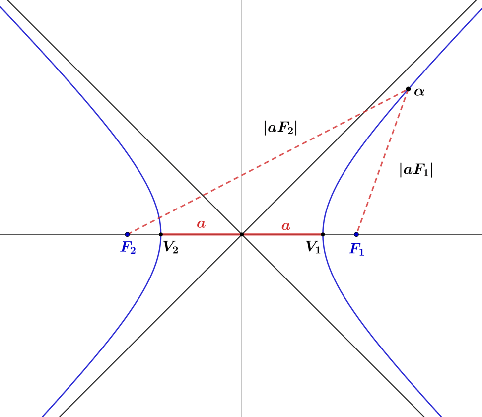
The Euclidean plane defines the hyperbola as a set of points with a semi-major axis , as the absolute difference between the fixed foci to the point on the hyperbola. The set of points is therefore, defined in set notation, as
(1.3.159)
where the invariant distance for all points on the hyperbola is equal to , referred to as the major axis. In Figure 1.3.14, we plot a hyperbola centered at the origin, defined by the expression
(1.3.160)
where, in this case, . Like the twice differentiable equation for the unit circle, we can represent the unit hyperbola in the plane with the invariant expression
(1.3.161)
Figure 1.3.14 – The hyperbola , with the invariance.
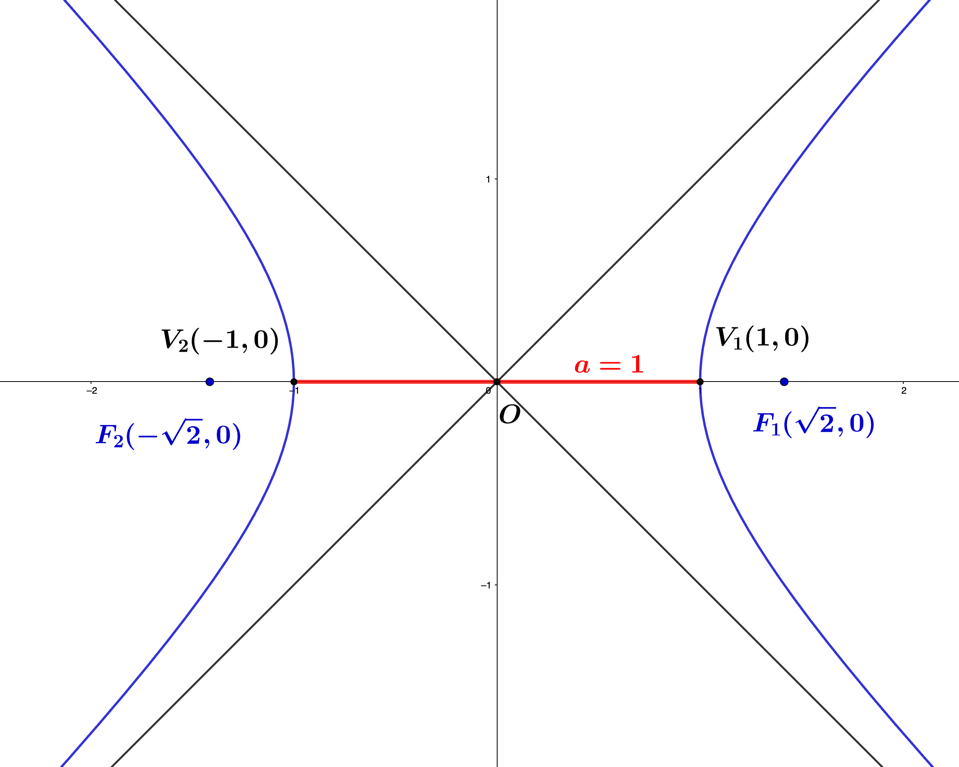
The unit hyperbola's curves are centered at the origin and oriented along the horizontal -axis, with semi-major axis values , vertices and , located at the coordinates and foci located at In the Euclidean plane, the unit hyperbola represents the plot seen in the Figure 1.3.15.
Figure 1.3.15 – The unit hyperbola , with semi-major axis , foci ,
vertices, and asymptotes in grey
The curvature and signed curvature formulas derived in Section 1.3.4, also hold for the hyperbola in the plane. Recalling the signed curvature formula
(1.3.162)
and its parametric form
(1.3.163)
To begin, we consider the curvature of the hyperbola in the plane by implicit differentiation its invariant form
(1.3.164)
the solve for
(1.3.165)
recalling that Next, we calculate the second-order derivative , to find
(1.3.166)
Taking the derivatives, we can now calculate the curvature of our unit hyperbola to be
(1.3.167)
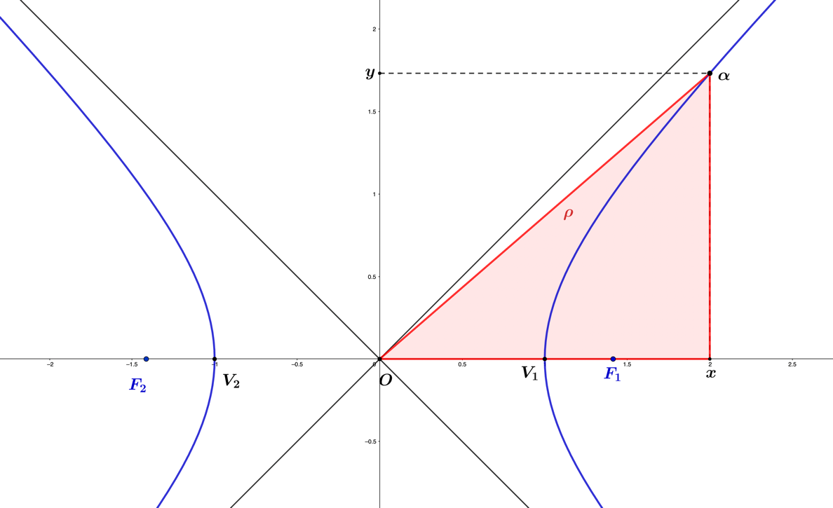
By defining , to represent the Euclidean distance from the center of the hyperbola to a point on the curve, the signed curvature equals
(1.3.168)
As an example, we consider the point on the unit hyperbola, finding equals
(1.3.169)
and thus, the signed curvature will equal
(1.3.170)
In Figure 1.3.16, the point is seen on the unit hyperbola, and the -segment represents the hypotenuse of the triangular polygon depicted in red.
The radius of curvature of the circular arc at a given point on the unit hyperbola, is
(1.3.171)
and for a defined point, , then equals
(1.3.172)
Figure 1.3.16 – The point on the unit hyperbola ,where
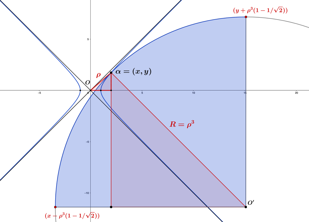
The radius of curvature vector , is tangent to the unit hyperbola at this point, and the circular arc will have its center , located at the point
(1.3.173)
Figure 1.3.17 – The point on the unit hyperbola , with a radius
of curvature, tangent to the unit hyperbola at the point,
Figure 1.3.17 demonstrates the radius of curvatureat the point , where a circular arc is shown with arclength
(1.3.174)
Next, we consider the parameterized form for the unit hyperbola in the plane,
(1.3.175)
and using the parameterized signed curvature formula
(1.3.176)
we evaluate, to find
(1.3.177)
Given that is the magnitude of the segment from the origin to the point located at ,
(1.3.178)
the signed curvature , becomes
(1.3.179)
which is the same result found for the non-parametrized form. Given that
(1.3.180)
we can express the signed curvature for the unit hyperbola, as
(1.3.181)
The highest magnitude of signed curvature for the unit hyperbola occurs for
(1.3.182)
and for the limit, as approaches infinity, equals the zero curvature of flat space
(1.3.183)
and using the hypotenuse , the following limit also approaches infinity,
(1.3.184)
A parallel exists between the curvatures of the hyperbola and the circle in the plane, where each curve will flatten with increasing values for their hypotenuse components . As , both curves become straight lines, defined with zero curvature
(1.3.185)
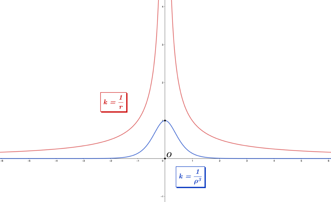
for which, the unit hyperbola will flatten much faster given the more significant degree of the term in its limit. In the following figure, we plot the functions for the signed curvatures of unit hyperbola , and the circle of radius in the plane , where we assume .
Figure 1.3.18 – Curvature functions for the unit hyperbola , and the circle
The plots show that the unit hyperbola's curvature quickly approaches the horizontal axis's zero curvature. In contrast, the curvature of the circle approaches the horizontal axis more slowly as we move away from the origin. As the radius of the circle decreases, the curvature increases and will approach an infinite curvature as the radius approaches zero
(1.3.186)
It is important to note that the hyperbola can also be scaled by a scalar radial component value, seen by adding the radial component to the parametrized function
(1.3.187)
and evaluating for the signed curvature
(1.3.188)
finding that the hyperbola's curvature also takes on the inverse radial characteristic like the circle.
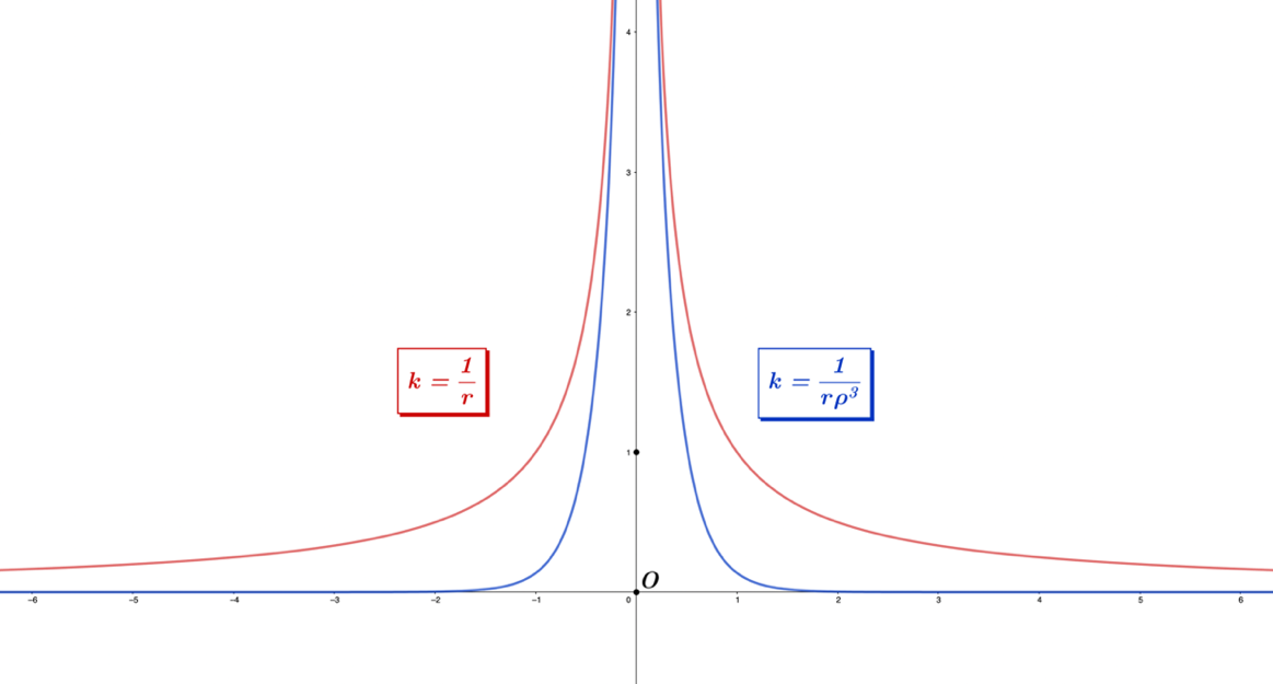
Figure 1.3.19 – Plots of the curvature functions for varying scalar radial values, . The curvature
of the hyperbola is seen in blue,, and the curvature of the circle is seen in red,
Comparing the plots for the curvature of the hyperbola and circle in Figure 1.3.19, shows that both will approach infinity for smaller scalar radial values of, but given the larger degree of the hyperbola's -term, its curvature function will approach infinity at a slower rate
(1.3.189)
This leads us to conclude that a more accurate way to consider curvature for hyperbolic and circular curves in the plane is to compare their unit representations and, respectively, the radially scaled curves from Figure 1.3.19. For the case of the unit curves, the circle's curvature magnitude does not change, , while the unit hyperbola's curvature magnitude may considerably change, given the power in the denominator of