1.3.8 Geometric Algebra

The geometric product is frequently used in physics, especially in the context of relativity. It is thus essential for the reader to conceptualize it coherently. It is defined for the product of two vectors $u,v$ , as the following

\begin{array}{r} uv = u \bullet v + \land v, \end{array}

(1.3.215)

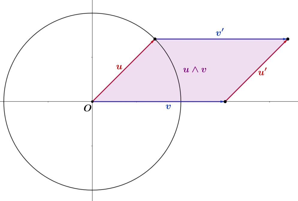
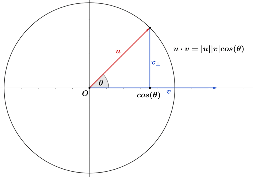
where $u \bullet v$ is the dot product of the vectors, representing the symmetric portion, and $u \land v$ is the wedge product, representing the antisymmetric portion. The geometric intuition that underscores the geometric product is that the vectors, $u$ , $v$ are parallel if their geometric product is equal to the dot product, while perpendicular if it is equal to the wedge product. As we can see below, the wedge product produces a bivector, representing a parallelogram with area and direction. In contrast, the dot product is the product of the vector's magnitudes and the cosine of the angle between them. We start by defining our $u$ and $v$ vectors

\begin{array}{r} u = \begin{pmatrix} a \\ b \end{pmatrix},\ \ v = \begin{pmatrix} c \\ d \end{pmatrix}, \end{array}

(1.3.216)

for which, the dot product of these two vectors is

\begin{array}{r} u \bullet v = ac + bd. \end{array}

(1.3.217)

The wedge product makes use of unit basis vectors, seen by using the example of the two-dimensional real plane, where the basis vectors $e_{1},e_{2}$ , can be represented, as

\begin{array}{r} e_{1} = \begin{pmatrix} 1 \\ 0 \end{pmatrix},\ \ e_{2} = \begin{pmatrix} 0 \\ 1 \end{pmatrix}. \end{array}

(1.3.218)

We proceed to consider the wedge product between the vectors $u$ , $v$ , as follows

u \land v = \left( e_{1}a + e_{2}b \right) \land \left( e_{1}c + e_{2}d \right)

\begin{array}{r} = ace_{1} \land e_{1} + ade_{1} \land e_{2} + bce_{2} \land e_{1} + bde_{2} \land e_{2} = (ad - bc)e_{1} \land e_{2}, \end{array}

(1.3.219)

where it is noted for the wedge product of unit basis vectors

\begin{array}{r} e_{1} \land e_{1} = e_{2} \land e_{2} = 0, \end{array}

(1.3.220)

\begin{array}{r} e_{1} \land e_{2} = - e_{2} \land e_{1}. \end{array}

(1.3.221)

Figure 1.3.20 – The wedge product of two vectors $u$ and $v$ $(u \land v).$

Figure 1.3.21 – The dot product of two vectors $u$ and $v$ , $(u \bullet v).$

The intuition for these unit basis vector products relates to the determinant and the orientated area of the parallelogram, which forms by the composition of the two vectors. The unit basis vectors forming wedge products can be combined into a matrix from, and assessed, as follows

\begin{array}{r} e_{1} \land e_{2} = det\begin{pmatrix} 1 & 0 \\ 0 & 1 \end{pmatrix} = 1, \end{array}

(1.3.222)

\begin{array}{r} e_{2} \land e_{1} = \det\begin{pmatrix} 0 & 1 \\ 1 & 0 \end{pmatrix} = - 1, \end{array}

(1.3.223)

\begin{array}{r} e_{1} \land e_{1} = \det\begin{pmatrix} 1 & 1 \\ 0 & 0 \end{pmatrix} = 0, \end{array}

(1.3.224)

\begin{array}{r} e_{2} \land e_{2} = \det{\begin{pmatrix} 0 & 0 \\ 1 & 1 \end{pmatrix} = 0.} \end{array}

(1.3.225)

The various dot products between the unit basis vectors then equal the following

\begin{array}{r} e_{1} \bullet e_{2} = (1,0)(0,1)^{T} = 0, \end{array}

(1.3.226)

\begin{array}{r} e_{2} \bullet e_{1} = (0,1)(1,0)^{T} = 0, \end{array}

(1.3.227)

\begin{array}{r} e_{1} \bullet e_{1} = (1,0)(1,0)^{T} = 1, \end{array}

(1.3.228)

\begin{array}{r} e_{2} \bullet e_{2} = (0,1)(0,1)^{T} = 1, \end{array}

(1.3.229)

which, in the context of their respective wedge products, the geometric products of the parallel unit basis vectors are uniquely the result of the dot product

\begin{array}{r} e_{1} \bullet e_{1} + e_{1} \land e_{1} = 1 + 0, \end{array}

(1.3.230)

\begin{array}{r} e_{2} \bullet e_{2} + e_{2} \land e_{2} = 1 + 0. \end{array}

(1.3.231)

In turn, the perpendicular unit basis vectors are solely the result of the wedge product portion of the geometric product

\begin{array}{r} e_{1} \bullet e_{2} + e_{1} \land e_{2} = 0 + 1, \end{array}

(1.3.232)

\begin{array}{r} e_{2} \bullet e_{1} + e_{2} \land e_{1} = 0 - 1. \end{array}

(1.3.233)

mindful that the wedge product results are bivectors. The notation $I$ is commonly used to denote the following wedge products

\begin{array}{r} I = e_{1} \land e_{2}, \end{array}

(1.3.234)

\begin{array}{r} - I = e_{2} \land e_{1}, \end{array}

(1.3.235)

which is isomorphic with the imaginary number $i$ in the complex plane. This isomorphism is appreciated by squaring the bivector

I^{2} = \left( e_{1} \land e_{2} \right)\left( e_{1} \land e_{2} \right) = e_{1}e_{2}e_{1}e_{2}

\begin{array}{r} = - e_{2}e_{1}e_{1}e_{2} = - e_{2}e_{2} = - 1, \end{array}

(1.3.236)

where we use the fact that, the wedge product of the two basis vectors equals their geometric product

\begin{array}{r} e_{1} \land e_{2} = e_{1}e_{2}, \end{array}

(1.3.237)

since they are perpendicular, are therefore, have a dot product equal to zero. So, the geometric product of two basis vectors can have four different components: a scalar, two vectors $e_{1},e_{2}$ , and a bivector $e_{1} \land e_{2}.$ We start with an example using the geometric product to project a vector $v$

\begin{array}{r} v = \left( e_{1}\left( \frac{e^{It}}{2} \right),e_{2}\left( \frac{e^{- It}}{2} \right) \right), \end{array}

(1.3.238)

comprised of exponential function components oriented in each basis, and then define the simple basis vector $u$

\begin{array}{r} u = \left( e_{1},e_{2} \right). \end{array}

(1.3.239)

Next, we take the geometric product of the two vectors, as $uv$ , being comprised of the sums of the dot and wedge products

\begin{array}{r} uv = u \bullet v + u \land v, \end{array}

(1.3.240)

finding the dot product equals

u \bullet v = \left( e_{1},e_{2} \right) \bullet \left( e_{1}\left( \frac{e^{It}}{2} \right),e_{2}\left( \frac{e^{- It}}{2} \right) \right)

\begin{array}{r} = e_{1} \bullet e_{1}\left( \frac{e^{It}}{2} \right) + e_{2} \bullet e_{2}\left( \frac{e^{- It}}{2} \right) = \frac{e^{It} + e^{- It}}{2}. \end{array}

(1.3.241)

This expression should look familiar, given that it is isomorphic with the complex-valued identity for the cosine function, seen by expanding and simplifying

\begin{array}{r} \frac{e^{It} + e^{- It}}{2} = \frac{1}{2}\left( \cos(t) + Isin(t) + \cos(t) - Isin(t) \right) = \cos(t), \end{array}

(1.3.242)

and this is the expected result for $u \bullet v$ . We proceed, by evaluating the wedge product,

u \land v = \left( e_{1} + e_{2} \right) \land \left( e_{1}\left( \frac{e^{It}}{2} \right) + e_{2}\left( \frac{e^{- It}}{2} \right) \right)

= e_{1} \land e_{1}\left( \frac{e^{It}}{2} \right) + e_{1} \land e_{2}\left( \frac{e^{- It}}{2} \right) + e_{2} \land e_{1}\left( \frac{e^{It}}{2} \right) + e_{2} \land e_{2}\left( \frac{e^{- It}}{2} \right)

\begin{array}{r} = e_{1} \land e_{2}\left( \frac{e^{- It}}{2} \right) + e_{2} \land e_{1}\left( \frac{e^{It}}{2} \right) = I\left( \frac{e^{- It}}{2} \right) - I\left( \frac{e^{It}}{2} \right) = \frac{e^{It} - e^{- It}}{2I}, \end{array}

(1.3.243)

which is an isomorphic complex-valued identity for the sine function. We expand this, and simplify

u \land v = \frac{I\left( \cos(t) - Isin(t) \right)}{2} - \frac{I\left( \cos(t) + Isin(t) \right)}{2}

\begin{array}{r} = \frac{{Icos}(t) + sin(t)}{2} - \frac{\left( {Icos}(t) - sin(t) \right)}{2} = \sin(t), \end{array}

(1.3.244)

then add the dot and wedge products together, arriving at the result for the geometric product $uv$

\begin{array}{r} uv = \cos(t) + \sin(t). \end{array}

(1.3.245)

In this example, we chose to not distribute the bivector $I$ into the cosine and sine functions in the exponential, where for instance, when distributing $I$ , the product $e_{1}\left( \frac{e^{It}}{2} \right)$ would equal

\begin{array}{r} e_{1}\left( \frac{e^{It}}{2} \right) = e_{1}\left( \frac{\cos(t)}{2} + e_{1} \land e_{2}\frac{\sin(t)}{2} \right) = \frac{e_{1}\cos(t)}{2} + \frac{e_{2}\sin(t)}{2}. \end{array}

(1.3.246)

If we did so, the $e_{2}\sin(t)$ vector portion would then be placed into the $e_{2}$ basis position. In these cases, care must be taken given that the unit bases anticommute with wedge products. To demonstrate that distributing the bases for the vector $v$ at the onset is viable, we distribute the $e_{2}$ basis into the exponential for the other $e_{2}\left( \frac{e^{- It}}{2} \right)$ vector component

\begin{array}{r} e_{2}\left( \frac{e^{- It}}{2} \right) = e_{2}\left( \frac{\cos(t)}{2} + e_{2} \land e_{1}\frac{\sin(t)}{2} \right) = \frac{e_{2}\cos(t)}{2} + \frac{e_{1}\sin(t)}{2}, \end{array}

(1.3.247)

then express $v^{'}$ , as the components ordered by basis

\begin{array}{r} v^{'} = \begin{pmatrix} \frac{e_{1}}{2}\left( \cos(t) + \sin(t) \right) \\ \frac{e_{2}}{2}\left( \cos(t) + \sin(t) \right) \end{pmatrix}. \end{array}

(1.3.248)

Now, we evaluate the product $uv^{'}$

\begin{array}{r} uv^{'} = u \bullet v^{'} + u \land v^{'}, \end{array}

(1.3.249)

starting with the dot product portion

\begin{array}{r} \left( e_{1},e_{2} \right)\ \bullet v^{'} = \cos(t) + \sin(t), \end{array}

(1.3.250)

whose result is due to the scalar portion $\left( \cos(t) + \sin(t) \right)$ being the same for both bases, and then the wedge product will equal zero

\begin{array}{r} \left( e_{1} + e_{2} \right) \land \left( \frac{e_{1}}{2} + \frac{e_{2}}{2} \right) = \frac{e_{1} \land e_{1} + e_{1} \land e_{2} + e_{2} \land e_{1} + e_{2} \land e_{2}}{2} = 0. \end{array}

(1.3.251)

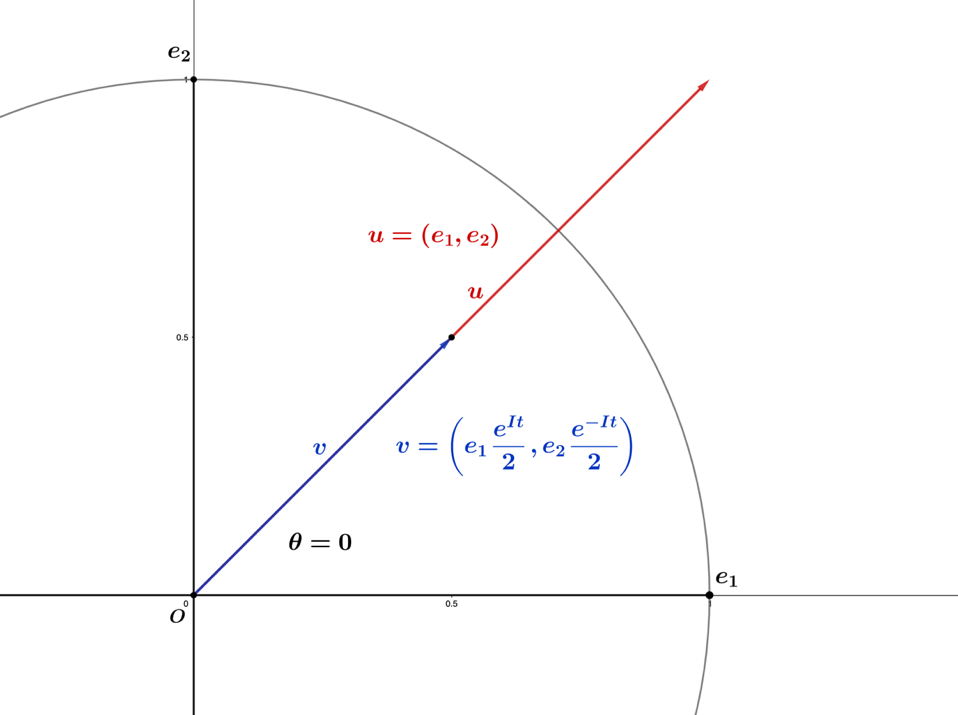
In Figure 1.3.22, the vectors $u$ , $v$ are parallel in orientation and therefore, have a geometric product defined solely by their dot product.

Figure 1.3.22 –Parallel vectors $u$ and $v$ with geometric product $uv = u \bullet v.$

In general, the geometric product should not be assumed to be commutative, given that the order of the product can result in a rotation in the opposite direction. To demonstrate, we switch the geometric product order from the previous example

\begin{array}{r} vu = v \bullet u + v \land u, \end{array}

(1.3.252)

then proceed to find the dot and wedge product portions, as follows

v \bullet u = \left( e_{1}\left( \frac{e^{It}}{2} \right),e_{2}\left( \frac{e^{- It}}{2} \right) \right) \bullet \left( e_{1},e_{2} \right) = \frac{e^{It}}{2} + \frac{e^{- It}}{2},

\begin{array}{r} v \land u = \left( e_{1}\left( \frac{e^{It}}{2} \right) + e_{2}\left( \frac{e^{- It}}{2} \right) \right) \land \left( e_{1},e_{2} \right) = e_{1} \land e_{2}\left( \frac{e^{It}}{2} \right) + e_{2} \land e_{1}\left( \frac{e^{- It}}{2} \right). \end{array}

(1.3.253)

The dot product is symmetric and, as expected, remains the same, while the antisymmetric wedge product has changed in sign when compared to the wedge product from $u \land v$ ,

\begin{array}{r} u \land v = e_{1} \land e_{2}\left( \frac{e^{- It}}{2} \right) + e_{2} \land e_{1}\left( \frac{e^{It}}{2} \right). \end{array}

(1.3.254)

So, it becomes clear that, $u \land v = - v \land u.$ The result of the reversed-order geometric product is

\begin{array}{r} vu = \cos(t) - \sin(t), \end{array}

(1.3.255)

where the change in the sign for the $\sin(t)$ value indicates a shift in the direction of rotation. Geometric algebra will be an essential tool when we start considering flat curvature and the functions that generate the asymptotic boundaries of the unit hyperbola.

Text size

Light or dark

Look