We have previously mentioned that the groups D 3 ℂ ⊞ D_{3\mathbb{C}}^{\boxplus} D 3 ℂ Δ D_{3\mathbb{C}}^{\Delta} 𝒴 \mathcal{Y}
{ ( A 0 0 0 A 0 0 0 A ) , ( C 0 0 0 C 0 0 0 A ) , ( A 0 0 0 C 0 0 0 C ) , ( C 0 0 0 A 0 0 0 C ) } ∈ Y 1 , k , \left\{ \begin{pmatrix}
A & 0 & 0 \\
0 & A & 0 \\
0 & 0 & A
\end{pmatrix},\begin{pmatrix}
C & 0 & 0 \\
0 & C & 0 \\
0 & 0 & A
\end{pmatrix},\begin{pmatrix}
A & 0 & 0 \\
0 & C & 0 \\
0 & 0 & C
\end{pmatrix},\begin{pmatrix}
C & 0 & 0 \\
0 & A & 0 \\
0 & 0 & C
\end{pmatrix} \right\} \in Y_{1,k}, { ( 0 A 0 0 0 A A 0 0 ) , ( 0 C 0 0 0 C A 0 0 ) , ( 0 A 0 0 0 C C 0 0 ) , ( 0 C 0 0 0 A C 0 0 ) } ∈ Y 2 , k , \left\{ \begin{pmatrix}
0 & A & 0 \\
0 & 0 & A \\
A & 0 & 0
\end{pmatrix},\begin{pmatrix}
0 & C & 0 \\
0 & 0 & C \\
A & 0 & 0
\end{pmatrix},\begin{pmatrix}
0 & A & 0 \\
0 & 0 & C \\
C & 0 & 0
\end{pmatrix},\begin{pmatrix}
0 & C & 0 \\
0 & 0 & A \\
C & 0 & 0
\end{pmatrix} \right\} \in Y_{2,k}, { ( 0 0 A A 0 0 0 A 0 ) , ( 0 0 A C 0 0 0 C 0 ) , ( 0 0 C A 0 0 0 C 0 ) , ( 0 0 A C 0 0 0 C 0 ) } ∈ Y 3 , k , \begin{array}{r}
\left\{ \begin{pmatrix}
0 & 0 & A \\
A & 0 & 0 \\
0 & A & 0
\end{pmatrix},\begin{pmatrix}
0 & 0 & A \\
C & 0 & 0 \\
0 & C & 0
\end{pmatrix},\begin{pmatrix}
0 & 0 & C \\
A & 0 & 0 \\
0 & C & 0
\end{pmatrix},\begin{pmatrix}
0 & 0 & A \\
C & 0 & 0 \\
0 & C & 0
\end{pmatrix} \right\} \in Y_{3,k},
\end{array} (1.4.125) and axis numbered determinants. There is a conspicuous absence of the elements ∈ 𝒴 \in \mathcal{Y} cone numbered determinant values, which define the D 3 ℂ ⊞ , D 3 ℂ Δ D_{3\mathbb{C}}^{\boxplus},D_{3\mathbb{C}}^{\Delta} S 3 ℂ Δ S_{3\mathbb{C}}^{\Delta} 𝒴 \mathcal{Y} ⊂ \subset S 3 ℂ Δ S_{3\mathbb{C}}^{\Delta} axis and cone numbers , and in addition to the stated axis determinant forms, the inclusion of the cone determinant elements round out the subgroup,
{ ( C 0 0 0 C 0 0 0 C ) , ( C 0 0 0 A 0 0 0 A ) , ( A 0 0 0 A 0 0 0 C ) , ( A 0 0 0 C 0 0 0 A ) } ∈ Y 1 , k , \left\{ \begin{pmatrix}
C & 0 & 0 \\
0 & C & 0 \\
0 & 0 & C
\end{pmatrix},\begin{pmatrix}
C & 0 & 0 \\
0 & A & 0 \\
0 & 0 & A
\end{pmatrix},\begin{pmatrix}
A & 0 & 0 \\
0 & A & 0 \\
0 & 0 & C
\end{pmatrix},\begin{pmatrix}
A & 0 & 0 \\
0 & C & 0 \\
0 & 0 & A
\end{pmatrix} \right\} \in Y_{1,k}, { ( 0 C 0 0 0 C C 0 0 ) , ( 0 C 0 0 0 A A 0 0 ) , ( 0 A 0 0 0 A C 0 0 ) , ( 0 A 0 0 0 C A 0 0 ) } ∈ Y 2 , k , \left\{ \begin{pmatrix}
0 & C & 0 \\
0 & 0 & C \\
C & 0 & 0
\end{pmatrix},\begin{pmatrix}
0 & C & 0 \\
0 & 0 & A \\
A & 0 & 0
\end{pmatrix},\begin{pmatrix}
0 & A & 0 \\
0 & 0 & A \\
C & 0 & 0
\end{pmatrix},\begin{pmatrix}
0 & A & 0 \\
0 & 0 & C \\
A & 0 & 0
\end{pmatrix} \right\} \in Y_{2,k}, { ( 0 0 C C 0 0 0 C 0 ) , ( 0 0 C A 0 0 0 A 0 ) , ( 0 0 A A 0 0 0 C 0 ) , ( 0 0 A C 0 0 0 A 0 ) } ∈ Y 3 , k . \begin{array}{r}
\left\{ \begin{pmatrix}
0 & 0 & C \\
C & 0 & 0 \\
0 & C & 0
\end{pmatrix},\begin{pmatrix}
0 & 0 & C \\
A & 0 & 0 \\
0 & A & 0
\end{pmatrix},\begin{pmatrix}
0 & 0 & A \\
A & 0 & 0 \\
0 & C & 0
\end{pmatrix},\begin{pmatrix}
0 & 0 & A \\
C & 0 & 0 \\
0 & A & 0
\end{pmatrix} \right\} \in Y_{3,k}.
\end{array} (1.4.126) For the 𝒴 \mathcal{Y}
| 𝒴 j − λ I | = 0 , \begin{array}{r}
\left| \mathcal{Y}_{j} - \lambda I \right| = 0,
\end{array} (1.4.127) and solving for the characteristic polynomials of 𝒴 j \mathcal{Y}_{j} 𝒴 1 \mathcal{Y}_{1}
det ( − λ + a 0 0 0 − λ + b 0 C 0 − λ + c ) = 0 → ( − λ + a ) ( − λ + b ) ( − λ + c ) = 0 → λ = a , b , c , \begin{array}{r}
\det\begin{pmatrix}
- \lambda + a & 0 & 0 \\
0 & - \lambda + b & 0 \\
C & 0 & - \lambda + c
\end{pmatrix} = 0 \rightarrow ( - \lambda + a)( - \lambda + b)( - \lambda + c) = 0 \rightarrow \ \lambda = a,b,c,
\end{array} (1.4.128) for 𝒴 2 \mathcal{Y}_{2}
det ( − λ a 0 0 − λ b c 0 − λ ) = 0 → λ 3 = − a b c , \begin{array}{r}
\det\begin{pmatrix}
- \lambda & a & 0 \\
0 & - \lambda & b \\
c & 0 & - \lambda
\end{pmatrix} = 0 \rightarrow \lambda^{3} = - abc,
\end{array} (1.4.129) whose terms a , b , c a,b,c cone number or axis number values, and ultimately, we find a similar result for the characteristic polynomial of 𝒴 3 \mathcal{Y}_{3}
det ( − λ 0 a b − λ 0 0 c − λ ) = 0 → λ 3 = − a b c . \begin{array}{r}
\det\begin{pmatrix}
- \lambda & 0 & a \\
b & - \lambda & 0 \\
0 & c & - \lambda
\end{pmatrix} = 0 \rightarrow \lambda^{3} = - abc.
\end{array} (1.4.130) Since the a , b , c a,b,c cone or an axis number , 𝒴 j \mathcal{Y}_{j}
λ ( 𝒴 j ) = { ± 1 , ± i , ± ( − 1 ) 1 4 , ± ( − 1 ) 3 4 } . \begin{array}{r}
\lambda\left( \mathcal{Y}_{j} \right) = \left\{ \pm 1, \pm i, \pm ( - 1)^{\frac{1}{4}}, \pm ( - 1)^{\frac{3}{4}} \right\}.
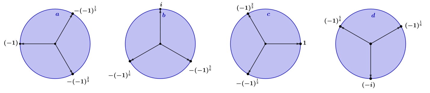
\end{array} (1.4.131) Figure 1.4.16 – λ ⊞ ( 𝒴 2 , 𝒴 3 ) \lambda^{\boxplus}\left( \mathcal{Y}_{2},\mathcal{Y}_{3} \right) ( ( − 1 ) 1 3 , − 1 , − ( − 1 ) 2 3 ) λ 3 = − 1 \left( ( - 1)^{\frac{1}{3}}, - 1,{- ( - 1)}^{\frac{2}{3}} \right)_{\lambda^{3} = - 1} ( i , − ( − 1 ) 1 6 , − ( − 1 ) 5 6 ) λ 3 = − i \left( i, - ( - 1)^{\frac{1}{6}}, - ( - 1)^{\frac{5}{6}} \right)_{\lambda^{3} = - i} c. ( 1 , ( − 1 ) 2 3 , − ( − 1 ) 1 3 ) λ 3 = 1 \left( 1,( - 1)^{\frac{2}{3}},{- ( - 1)}^{\frac{1}{3}} \right)_{\lambda^{3} = 1} , d. ( − i , ( − 1 ) 1 6 , ( − 1 ) 5 6 ) λ 3 = i \left( - i,( - 1)^{\frac{1}{6}},( - 1)^{\frac{5}{6}} \right)_{\lambda^{3} = i} .
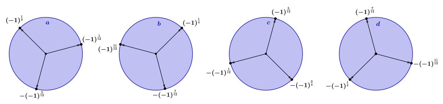
Figure 1.4.17 – λ Δ ( 𝒴 2 , 𝒴 3 ) \lambda^{\Delta}\left( \mathcal{Y}_{2},\mathcal{Y}_{3} \right) ( ( − 1 ) 1 12 , ( − 1 ) 3 4 , − ( − 1 ) 5 12 ) λ 3 = ( − 1 ) 1 4 \left( ( - 1)^{\frac{1}{12}},{( - 1)^{\frac{3}{4}}, - ( - 1)}^{\frac{5}{12}} \right)_{\lambda^{3} = ( - 1)^{\frac{1}{4}}} ( ( − 1 ) 1 4 , ( − 1 ) 11 12 , − ( − 1 ) 7 12 ) λ 3 = ( − 1 ) 3 4 \left( ( - 1)^{\frac{1}{4}},( - 1)^{\frac{11}{12}},{- ( - 1)}^{\frac{7}{12}} \right)_{\lambda^{3} = ( - 1)^{\frac{3}{4}}} c. ( ( − 1 ) 5 12 , − ( − 1 ) 1 12 , − ( − 1 ) 3 4 ) λ 3 = − ( − 1 ) 1 4 \left( ( - 1)^{\frac{5}{12}},{- ( - 1)}^{\frac{1}{12}},{- ( - 1)}^{\frac{3}{4}} \right)_{\lambda^{3} = {- ( - 1)}^{\frac{1}{4}}} , d. ( ( − 1 ) 7 12 , − ( − 1 ) 1 4 , − ( − 1 ) 11 12 ) λ 3 = − ( − 1 ) 3 4 \left( ( - 1)^{\frac{7}{12}}, - ( - 1)^{\frac{1}{4}}, - ( - 1)^{\frac{11}{12}} \right)_{\lambda^{3} = - ( - 1)^{\frac{3}{4}}} .
Comparing possible eigenvalues for 𝒴 2 , 𝒴 3 \mathcal{Y}_{2},\mathcal{Y}_{3} axis number determinants, having four possible values (Figure 1.4.16
λ ⊞ ( 𝒴 2 , 𝒴 3 ) = { ( − 1 , ( − 1 ) 1 3 , − ( − 1 ) 2 3 ) λ 3 = − 1 , ( i , − ( − 1 ) 1 6 , − ( − 1 ) 5 6 ) λ 3 = − i , ( 1 , , − ( − 1 ) 1 3 , ( − 1 ) 2 3 ) λ 3 = − 1 , ( − i , ( − 1 ) 1 6 , ( − 1 ) 5 6 ) λ 3 = − i } , \begin{array}{r}
\lambda^{\boxplus}\left( \mathcal{Y}_{2},\mathcal{Y}_{3} \right) = \left\{ \begin{array}{r}
\ \left( - 1,( - 1)^{\frac{1}{3}},{- ( - 1)}^{\frac{2}{3}} \right)_{\lambda^{3} = - 1},\ \ \ \left( i, - ( - 1)^{\frac{1}{6}}, - ( - 1)^{\frac{5}{6}} \right)_{\lambda^{3} = - i}, \\
\left( 1,{, - ( - 1)^{\frac{1}{3}},( - 1)}^{\frac{2}{3}} \right)_{\lambda^{3} = - 1},\ \ \ \left( - i,( - 1)^{\frac{1}{6}},( - 1)^{\frac{5}{6}} \right)_{\lambda^{3} = - i}
\end{array} \right\},
\end{array} (1.4.132) and 𝒴 2 , 𝒴 3 \mathcal{Y}_{2},\mathcal{Y}_{3} cone number determinants from the set of the four following values (Figure 1.4.17
λ Δ ( 𝒴 2 , 𝒴 3 ) = { ( ( − 1 ) 1 12 , ( − 1 ) 3 4 , − ( − 1 ) 5 12 ) λ 3 = ( − 1 ) 1 4 , ( ( − 1 ) 1 4 , ( − 1 ) 11 12 , − ( − 1 ) 7 12 ) λ 3 = ( − 1 ) 3 4 , ( ( − 1 ) 5 12 , − ( − 1 ) 1 12 , − ( − 1 ) 3 4 ) λ 3 = − ( − 1 ) 1 4 , ( ( − 1 ) 7 12 , − ( − 1 ) 1 4 , − ( − 1 ) 11 12 ) λ 3 = − ( − 1 ) 3 4 } . \begin{array}{r}
\lambda^{\Delta}\left( \mathcal{Y}_{2},\mathcal{Y}_{3} \right) = \left\{ \begin{array}{r}
\left( ( - 1)^{\frac{1}{12}},{( - 1)^{\frac{3}{4}}, - ( - 1)}^{\frac{5}{12}} \right)_{\lambda^{3} = ( - 1)^{\frac{1}{4}}},\ \ \ \left( ( - 1)^{\frac{1}{4}},( - 1)^{\frac{11}{12}},{- ( - 1)}^{\frac{7}{12}} \right)_{\lambda^{3} = ( - 1)^{\frac{3}{4}}}, \\
\ \\
\ \left( ( - 1)^{\frac{5}{12}},{- ( - 1)}^{\frac{1}{12}},{- ( - 1)}^{\frac{3}{4}} \right)_{\lambda^{3} = {- ( - 1)}^{\frac{1}{4}}},\ \ \ \left( ( - 1)^{\frac{7}{12}}, - ( - 1)^{\frac{1}{4}}, - ( - 1)^{\frac{11}{12}} \right)_{\lambda^{3} = - ( - 1)^{\frac{3}{4}}}
\end{array} \right\}.
\end{array} (1.4.133) When considering possible eigenvalues of 𝒴 1 \mathcal{Y}_{1} a , b , c a,b,c
( − λ + a ) ( − λ + b ) ( − λ + c ) = 0 → λ = a , b , c , \begin{array}{r}
( - \lambda + a)( - \lambda + b)( - \lambda + c) = 0 \rightarrow \ \lambda = a,b,c,
\end{array} (1.4.134) meaning, we can have mixed values in the form of cone numbers and axis numbers . This is quite different than the 𝒴 2 , 𝒴 3 \mathcal{Y}_{2},\mathcal{Y}_{3} 𝒴 1 \mathcal{Y}_{1}