We are now well versed in the association that integration has with exponentiation and the association that differentiation, the inverse of integration, has with the logarithm. It is important to remember that the infinite number of tangent spaces that reside on the boundary of the infinite sphere of tangent spaces are Lie algebra representations, containing all the information of the whole infinite symmetry group S 3 ℂ ∞ S_{3\mathbb{C}}^{\infty} ∈ 𝔰 3 ℂ ∞ \in \mathfrak{s}_{3\mathbb{C}}^{\infty} e θ r [ m ] e^{\theta_{r}^{\lbrack m\rbrack}} θ r [ m ] ∈ ℂ m \theta_{r}^{\lbrack m\rbrack} \in \mathbb{C}^{m} θ r [ m ] \theta_{r}^{\lbrack m\rbrack} e i θ j ∈ ℂ , | e i θ j | = 1 e^{i\theta_{j}}\in \mathbb{C},\left| e^{i\theta_{j}} \right| = 1 X 1 X_{1}
θ r j [ X 1 ] = ( r 1 e i θ 1 0 0 0 0 r 2 e i θ 2 0 r 3 e i θ 3 0 ) = ( ( a 1 + i b 1 ) 0 0 0 0 ( a 2 + i b 2 ) 0 ( a 3 + i b 3 ) 0 ) = ( z 1 0 0 0 0 z 2 0 z 3 0 ) , \begin{array}{r}
\theta_{r_{j}}^{\left\lbrack X_{1} \right\rbrack} = \begin{pmatrix}
r_{1}e^{i\theta_{1}} & 0 & 0 \\
0 & 0 & r_{2}e^{i\theta_{2}} \\
0 & r_{3}e^{i\theta_{3}} & 0
\end{pmatrix} = \begin{pmatrix}
\left( a_{1} + ib_{1} \right) & 0 & 0 \\
0 & 0 & \left( a_{2} + ib_{2} \right) \\
0 & \left( a_{3} + ib_{3} \right) & 0
\end{pmatrix} = \begin{pmatrix}
z_{1} & 0 & 0 \\
0 & 0 & z_{2} \\
0 & z_{3} & 0
\end{pmatrix},
\end{array} (1.6.251) for a j , b j ∈ ℝ , z j ∈ ℂ a_{j},b_{j}\in \mathbb{R}\ ,\ z_{j}\in \mathbb{C} θ r j [ m ] \theta_{r_{j}}^{\lbrack m\rbrack} X 1 X_{1}
Z j [ R e ( D 3 𝕫 ( X 1 ) ) ] = R e ( z 1 0 0 0 0 z 2 0 z 3 0 ) = ( a 1 0 0 0 0 a 2 0 a 3 0 ) , \begin{array}{r}
Z_{j}^{\left\lbrack {Re(D}_{3\mathbb{z}}\left( X_{1} \right)) \right\rbrack} = Re\begin{pmatrix}
z_{1} & 0 & 0 \\
0 & 0 & z_{2} \\
0 & z_{3} & 0
\end{pmatrix} = \begin{pmatrix}
a_{1} & 0 & 0 \\
0 & 0 & a_{2} \\
0 & a_{3} & 0
\end{pmatrix},
\end{array} (1.6.252) Z j [ i × I m ( D 3 𝕫 ( X 1 ) ) ] = i × I m ( z 1 0 0 0 0 z 2 0 z 3 0 ) = ( i b 1 0 0 0 0 i b 2 0 i b 3 0 ) , \begin{array}{r}
Z_{j}^{\left\lbrack {i \times Im(D}_{3\mathbb{z}}\left( X_{1} \right)) \right\rbrack} = i \times Im\begin{pmatrix}
z_{1} & 0 & 0 \\
0 & 0 & z_{2} \\
0 & z_{3} & 0
\end{pmatrix} = \begin{pmatrix}
{ib}_{1} & 0 & 0 \\
0 & 0 & {ib}_{2} \\
0 & {ib}_{3} & 0
\end{pmatrix},
\end{array} (1.6.253) and in the polar form, as
θ r j [ D 3 𝕫 ( X 1 ) ] = ( r 1 e i θ 1 0 0 0 0 r 2 e i θ 2 0 r 3 e i θ 3 0 ) , \begin{array}{r}
\theta_{r_{j}}^{\left\lbrack D_{3\mathbb{z}}\left( X_{1} \right) \right\rbrack} = \begin{pmatrix}
r_{1}e^{i\theta_{1}} & 0 & 0 \\
0 & 0 & r_{2}e^{i\theta_{2}} \\
0 & r_{3}e^{i\theta_{3}} & 0
\end{pmatrix},
\end{array} (1.6.254) which can be decomposed into the product of its radial modulus matrix and spherical matrix group
θ r j [ D 3 𝕫 ( X 1 ) ] = ( r 1 0 0 0 r 2 0 0 0 r 3 ) ( e i θ 1 0 0 0 0 e i θ 2 0 e i θ 3 0 ) . \begin{array}{r}
\theta_{r_{j}}^{\left\lbrack D_{3\mathbb{z}}\left( X_{1} \right) \right\rbrack} = \begin{pmatrix}
r_{1} & 0 & 0 \\
0 & r_{2} & 0 \\
0 & 0 & r_{3}
\end{pmatrix}\begin{pmatrix}
e^{i\theta_{1}} & 0 & 0 \\
0 & 0 & e^{i\theta_{2}} \\
0 & e^{i\theta_{3}} & 0
\end{pmatrix}.
\end{array} (1.6.255) Note, the product result will change if the spherical group is right multiplied by the modulus matrix
( e i θ 1 0 0 0 0 e i θ 2 0 e i θ 3 0 ) ( r 1 0 0 0 r 2 0 0 0 r 3 ) = ( r 1 e i θ 1 0 0 0 0 r 3 e i θ 2 0 r 2 e i θ 3 0 ) , \begin{array}{r}
\begin{pmatrix}
e^{i\theta_{1}} & 0 & 0 \\
0 & 0 & e^{i\theta_{2}} \\
0 & e^{i\theta_{3}} & 0
\end{pmatrix}\begin{pmatrix}
r_{1} & 0 & 0 \\
0 & r_{2} & 0 \\
0 & 0 & r_{3}
\end{pmatrix} = \begin{pmatrix}
r_{1}e^{i\theta_{1}} & 0 & 0 \\
0 & 0 & r_{3}e^{i\theta_{2}} \\
0 & r_{2}e^{i\theta_{3}} & 0
\end{pmatrix},
\end{array} (1.6.256) where the moduli variables have swapped positions in the bottom-right 2 × 2 2 \times 2
The tangent space group θ r j [ D 3 𝕫 ( X 1 ) ] \theta_{r_{j}}^{\left\lbrack D_{3\mathbb{z}}\left( X_{1} \right) \right\rbrack} ln ( θ r j [ D 3 𝕫 ( X 1 ) ] ) \ln\left( \theta_{r_{j}}^{\left\lbrack D_{3\mathbb{z}}\left( X_{1} \right) \right\rbrack} \right) Z j [ D 3 𝕫 ( X 1 ) ] Z_{j}^{\left\lbrack D_{3\mathbb{z}}\left( X_{1} \right) \right\rbrack}
ln ( Z j [ D 3 𝕫 ( X 1 ) ] ) = ( ln ( z 1 ) 0 0 0 ln ( z 2 z 3 ) + ln ( − z 2 z 3 ) 2 z 2 z 2 z 3 ( ln ( z 2 z 3 ) − ln ( − z 2 z 3 ) 2 ) 0 z 3 z 2 z 3 ( ln ( z 2 z 3 ) − ln ( − z 2 z 3 ) 2 ) ( ln ( z 2 z 3 ) + ln ( − z 2 z 3 ) ) 2 ) . \begin{array}{r}
\ln{\left( Z_{j}^{\left\lbrack D_{3\mathbb{z}}\left( X_{1} \right) \right\rbrack} \right) = \begin{pmatrix}
\ln\left( z_{1} \right) & 0 & 0 \\
0 & \frac{\ln{\left( \sqrt{z_{2}z_{3}} \right) + \ln\left( - \sqrt{z_{2}z_{3}} \right)}}{2} & \frac{z_{2}}{\sqrt{z_{2}z_{3}}}\left( \frac{\ln{\left( \sqrt{z_{2}z_{3}} \right) - \ln\left( - \sqrt{z_{2}z_{3}} \right)}}{2} \right) \\
0 & \frac{z_{3}}{\sqrt{z_{2}z_{3}}}\left( \frac{\ln{\left( \sqrt{z_{2}z_{3}} \right) - \ln\left( - \sqrt{z_{2}z_{3}} \right)}}{2} \right) & \frac{\left( \ln{\left( \sqrt{z_{2}z_{3}} \right) + \ln\left( - \sqrt{z_{2}z_{3}} \right)} \right)}{2}
\end{pmatrix}}.
\end{array} (1.6.257) The matrix exponential mapping of the Lie algebra Z j [ D 3 𝕫 ( X 1 ) ] Z_{j}^{\left\lbrack D_{3\mathbb{z}}\left( X_{1} \right) \right\rbrack} G ( Z j [ D 3 𝕫 ( X 1 ) ] ) = exp ( exp ( ln ( Z j [ D 3 𝕫 ( X 1 ) ] ) ) ) G\left( Z_{j}^{\left\lbrack D_{3\mathbb{z}}\left( X_{1} \right) \right\rbrack} \right) = \exp\left( \exp\left( \ln\left( Z_{j}^{\left\lbrack D_{3\mathbb{z}}\left( X_{1} \right) \right\rbrack} \right) \right) \right)
G ( Z j [ D 3 𝕫 ( X 1 ) ] ) = ( e z 1 0 0 0 cosh ( z 2 z 3 ) z 2 z 2 z 3 sinh ( z 2 z 3 ) 0 z 3 z 2 z 3 sinh ( z 2 z 3 ) cosh ( z 2 z 3 ) ) . \begin{array}{r}
G\left( Z_{j}^{\left\lbrack D_{3\mathbb{z}}\left( X_{1} \right) \right\rbrack} \right) = \begin{pmatrix}
e^{z_{1}} & 0 & 0 \\
0 & \cosh\left( \sqrt{z_{2}z_{3}} \right) & \frac{z_{2}}{\sqrt{{z_{2}z}_{3}}}\sinh\left( \sqrt{z_{2}z_{3}} \right) \\
0 & \frac{z_{3}}{\sqrt{{z_{2}z}_{3}}}\sinh\left( \sqrt{z_{2}z_{3}} \right) & \cosh\left( \sqrt{z_{2}z_{3}} \right)
\end{pmatrix}.
\end{array} (1.6.258) Conversely, the subtangent space is the result of the two-fold logarithm mapping of the Lie group ln ( ln ( G ( Z j [ D 3 𝕫 ( X 1 ) ] ) ) ) \ln(\ln\left( G\left( Z_{j}^{\left\lbrack D_{3\mathbb{z}}\left( X_{1} \right) \right\rbrack} \right) \right)) G ( Z j [ D 3 𝕫 ( X 1 ) ] ) G\left( Z_{j}^{\left\lbrack D_{3\mathbb{z}}\left( X_{1} \right) \right\rbrack} \right) z 2 z 3 \sqrt{z_{2}z_{3}}
z 2 z 3 = r 2 e i θ 2 × r 3 e i θ 3 \sqrt{z_{2}z_{3}} = \sqrt{r_{2}e^{i\theta_{2}}{\times r}_{3}e^{i\theta_{3}}} = ( e ln ( r 2 ) + i θ 2 × e ln ( r 3 ) + i θ 3 ) 1 2 = ( e ln ( r 2 r 3 ) + i ( θ 2 + θ 3 ) ) 1 2 = \left( e^{\ln\left( r_{2} \right) + i\theta_{2}}{\times e}^{\ln\left( r_{3} \right) + i\theta_{3}} \right)^{\frac{1}{2}} = \left( e^{\ln\left( r_{2}r_{3} \right) + i\left( \theta_{2} + \theta_{3} \right)} \right)^{\frac{1}{2}} = e 1 2 ( ln ( r 2 r 3 ) + i ( θ 2 + θ 3 ) ) = r 2 r 3 e i ( θ 2 2 + θ 3 2 ) . \begin{array}{r}
= e^{\frac{1}{2}\left( \ln\left( r_{2}r_{3} \right) + i\left( \theta_{2} + \theta_{3} \right) \right)} = \sqrt{r_{2}r_{3}}e^{i\left( \frac{\theta_{2}}{2} + \frac{\theta_{3}}{2} \right)}.
\end{array} (1.6.259) Next, using the constant z 3 z 2 z 3 \frac{z_{3}}{\sqrt{{z_{2}z}_{3}}}
z 3 z 2 z 3 = r 3 e i θ 3 r 2 r 3 e i ( θ 2 2 + θ 3 2 ) = r 3 r 2 r 3 ( e i θ 3 × e − i ( θ 2 2 + θ 3 2 ) ) = r 3 r 2 r 3 ( e i ( θ 3 2 − θ 2 2 ) ) , \begin{array}{r}
\frac{z_{3}}{\sqrt{{z_{2}z}_{3}}} = \frac{r_{3}e^{i\theta_{3}}}{\sqrt{r_{2}r_{3}}e^{i\left( \frac{\theta_{2}}{2} + \frac{\theta_{3}}{2} \right)}} = \frac{r_{3}}{\sqrt{r_{2}r_{3}}}\left( e^{i\theta_{3}} \times e^{- i\left( \frac{\theta_{2}}{2} + \frac{\theta_{3}}{2} \right)} \right) = \frac{r_{3}}{\sqrt{r_{2}r_{3}}}\left( e^{i\left( \frac{\theta_{3}}{2} - \frac{\theta_{2}}{2} \right)} \right),
\end{array} (1.6.260) and for r 3 , r 2 ∈ ℝ + r_{3},r_{2} \in \mathbb{R}^{+} z 3 z 2 z 3 \frac{z_{3}}{\sqrt{{z_{2}z}_{3}}}
r 3 r 2 r 3 ( e i ( θ 3 2 − θ 2 2 ) ) = r 3 r 2 ( e i ( θ 3 2 − θ 2 2 ) ) . \begin{array}{r}
\frac{r_{3}}{\sqrt{r_{2}r_{3}}}\left( e^{i\left( \frac{\theta_{3}}{2} - \frac{\theta_{2}}{2} \right)} \right) = \sqrt{\frac{r_{3}}{r_{2}}}\left( e^{i\left( \frac{\theta_{3}}{2} - \frac{\theta_{2}}{2} \right)} \right).
\end{array} (1.6.261) Given θ r j [ D 3 𝕫 ( X 1 ) ] = Z j [ D 3 𝕫 ( X 1 ) ] \theta_{r_{j}}^{\left\lbrack D_{3\mathbb{z}}\left( X_{1} \right) \right\rbrack} = Z_{j}^{\left\lbrack D_{3\mathbb{z}}\left( X_{1} \right) \right\rbrack} G ( Z j [ D 3 𝕫 ( X 1 ) ] ) = G ( θ r j [ D 3 𝕫 ( X 1 ) ] ) , G\left( Z_{j}^{\left\lbrack D_{3\mathbb{z}}\left( X_{1} \right) \right\rbrack} \right) = G\left( \theta_{r_{j}}^{\left\lbrack D_{3\mathbb{z}}\left( X_{1} \right) \right\rbrack} \right), G ( θ r j [ D 3 𝕫 ( X 1 ) ] ) G\left( \theta_{r_{j}}^{\left\lbrack D_{3\mathbb{z}}\left( X_{1} \right) \right\rbrack} \right)
G ( θ r j [ D 3 𝕫 ( X 1 ) ] ) = ( e r 1 e i θ 1 0 0 0 cosh ( r 2 r 3 e i ( θ 2 + θ 3 ) / 2 ) r 2 r 3 ( e i ( θ 2 2 − θ 3 2 ) ) sinh ( r 2 r 3 e i ( θ 2 2 + θ 3 2 ) ) 0 r 3 r 2 ( e i ( θ 3 2 − θ 2 2 ) ) sinh ( r 2 r 3 e i ( θ 2 2 + θ 3 2 ) ) cosh ( r 2 r 3 e i ( θ 2 + θ 3 ) / 2 ) ) . \begin{array}{r}
G\left( \theta_{r_{j}}^{\left\lbrack D_{3\mathbb{z}}\left( X_{1} \right) \right\rbrack} \right) = \begin{pmatrix}
e^{r_{1}e^{i\theta_{1}}} & 0 & 0 \\
0 & \cosh\left( \sqrt{r_{2}r_{3}}e^{i\left( \theta_{2} + \theta_{3} \right)/2} \right) & \sqrt{\frac{r_{2}}{r_{3}}}\left( e^{i\left( \frac{\theta_{2}}{2} - \frac{\theta_{3}}{2} \right)} \right)\sinh\left( \sqrt{r_{2}r_{3}}e^{i\left( \frac{\theta_{2}}{2} + \frac{\theta_{3}}{2} \right)} \right) \\
0 & \sqrt{\frac{r_{3}}{r_{2}}}\left( e^{i\left( \frac{\theta_{3}}{2} - \frac{\theta_{2}}{2} \right)} \right)\sinh\left( \sqrt{r_{2}r_{3}}e^{i\left( \frac{\theta_{2}}{2} + \frac{\theta_{3}}{2} \right)} \right) & \cosh\left( \sqrt{r_{2}r_{3}}e^{i\left( \theta_{2} + \theta_{3} \right)/2} \right)
\end{pmatrix}.
\end{array} (1.6.262) The matrix above represents the exponential mapping of the θ r j [ D 3 𝕫 ( X 1 ) ] \theta_{r_{j}}^{\left\lbrack D_{3\mathbb{z}}\left( X_{1} \right) \right\rbrack} ( θ r j [ D 3 𝕫 ( X 1 ) ] ) \left( \theta_{r_{j}}^{\left\lbrack D_{3\mathbb{z}}\left( X_{1} \right) \right\rbrack} \right)
det ( G ( θ r j [ D 3 𝕫 ( X 1 ) ] ) ) = e r 1 e i θ 1 ( ( cosh ( r 2 r 3 e i ( θ 2 + θ 3 ) 2 ) ) 2 − ( r 3 r 2 ( e i ( θ 3 2 − θ 2 2 ) ) sinh ( r 2 r 3 e i ( θ 2 2 + θ 3 2 ) ) × r 2 r 3 ( e i ( θ 2 2 − θ 3 2 ) ) sinh ( r 2 r 3 e i ( θ 2 2 + θ 3 2 ) ) ) ) \det\left( G\left( \theta_{r_{j}}^{\left\lbrack D_{3\mathbb{z}}\left( X_{1} \right) \right\rbrack} \right) \right) = e^{r_{1}e^{i\theta_{1}}}\left( \begin{array}{r}
\left( \cosh\left( \sqrt{r_{2}r_{3}}e^{\frac{i\left( \theta_{2} + \theta_{3} \right)}{2}} \right) \right)^{2} \\
- \ \left( \sqrt{\frac{r_{3}}{r_{2}}}\left( e^{i\left( \frac{\theta_{3}}{2} - \frac{\theta_{2}}{2} \right)} \right)\sinh\left( \sqrt{r_{2}r_{3}}e^{i\left( \frac{\theta_{2}}{2} + \frac{\theta_{3}}{2} \right)} \right) \times \sqrt{\frac{r_{2}}{r_{3}}}\left( e^{i\left( \frac{\theta_{2}}{2} - \frac{\theta_{3}}{2} \right)} \right)\sinh\left( \sqrt{r_{2}r_{3}}e^{i\left( \frac{\theta_{2}}{2} + \frac{\theta_{3}}{2} \right)} \right) \right)
\end{array} \right) = e r 1 e i θ 1 ( ( cosh ( r 2 r 3 e i ( θ 2 + θ 3 ) 2 ) ) 2 − ( sinh ( r 2 r 3 e i ( θ 2 2 + θ 3 2 ) ) ) 2 ) = e r 1 e i θ 1 ( 1 ) = e r 1 e i θ 1 , \begin{array}{r}
= e^{r_{1}e^{i\theta_{1}}}\left( \begin{array}{r}
\left( \cosh\left( \sqrt{r_{2}r_{3}}e^{\frac{i\left( \theta_{2} + \theta_{3} \right)}{2}} \right) \right)^{2} - \left( \sinh\left( \sqrt{r_{2}r_{3}}e^{i\left( \frac{\theta_{2}}{2} + \frac{\theta_{3}}{2} \right)} \right) \right)
\end{array}^{2} \right) = e^{r_{1}e^{i\theta_{1}}}(1) = e^{r_{1}e^{i\theta_{1}}},
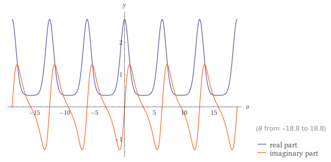
\end{array} (1.6.263) where the determinate equals the axis value e r 1 e i θ 1 , e^{r_{1}e^{i\theta_{1}}}, e z 1 e^{z_{1}} r 1 e i θ 1 = z 1 {r_{1}e^{i\theta_{1}} = z}_{1} r 1 = 1 r_{1} = 1 e e i θ 1 e^{e^{i\theta_{1}}} θ 1 \theta_{1} e e θ 1 = 2 π k \theta_{1} = 2\pi k k ∈ ℤ k\in \mathbb{Z} e − 1 ≈ 0.3679 e^{- 1} \approx 0.3679 θ 1 = π k \theta_{1} = \pi k k ∈ ℤ k\in \mathbb{Z} e i ≈ ( 0.5403 + 0.8415 i ) e^{i} \approx (0.5403 + 0.8415i) θ 1 = ( π 2 + 2 π k ) \theta_{1} = \left( \frac{\pi}{2} + 2\pi k \right) k ∈ ℤ k\in \mathbb{Z} e − t ≈ ( 0.5403 − 0.8415 i ) e^{- t} \approx (0.5403 - 0.8415i) θ 1 = ( 3 π 2 + 2 π k ) \theta_{1} = \left( \frac{3\pi}{2} + 2\pi k \right) k ∈ ℤ k\in \mathbb{Z} G ( θ 1 [ D 3 𝕫 ( X 1 ) ] ) G\left( \theta_{1}^{\left\lbrack D_{3\mathbb{z}}\left( X_{1} \right) \right\rbrack} \right) Figure 1.6.24
Figure 1.6.24 – Plot of det ( G ( θ 1 [ D 3 𝕫 ( X 1 ) ] ) ) = e e i θ 1 . \det\left( G\left( \theta_{1}^{\left\lbrack D_{3\mathbb{z}}\left( X_{1} \right) \right\rbrack} \right) \right) = e^{e^{i\theta_{1}}}. It is important to notice that the peaks and troughs for the real and imaginary waveforms are equal to the identity when considered as products, since e 1 e − 1 = ϵ e^{1}e^{- 1} = \epsilon e i e − i = ϵ e^{i}e^{- i} = \epsilon G ( θ r j [ D 3 𝕫 ( X 1 ) ] ) G\left( \theta_{r_{j}}^{\left\lbrack D_{3\mathbb{z}}\left( X_{1} \right) \right\rbrack} \right)
sinh ( r e i θ ) = cos ( r s i n ( θ ) ) sinh ( r c o s ( θ ) ) + i s i n ( r s i n ( θ ) ) cosh ( r c o s ( θ ) ) , \begin{array}{r}
{\sinh\left( re^{i\theta} \right) =}{\cos{\left( rsin(\theta) \right)\sinh{\left( rcos(\theta) \right) + isin\left( rsin(\theta) \right)\cosh\left( rcos(\theta) \right)}}},
\end{array} (1.6.264) cosh ( r e i θ ) = cos ( r s i n ( θ ) ) cosh ( r c o s ( θ ) ) + i s i n ( r s i n ( θ ) ) sinh ( r c o s ( θ ) ) , \begin{array}{r}
\cosh\left( re^{i\theta} \right) = \cos{\left( rsin(\theta) \right)\cosh{\left( rcos(\theta) \right) + isin\left( rsin(\theta) \right)\sinh\left( rcos(\theta) \right)}},
\end{array} (1.6.265) and substitute r = r 2 r 3 r = \sqrt{r_{2}r_{3}} e i θ = e i ( θ 2 + θ 3 ) / 2 , e^{i\theta} = e^{i\left( \theta_{2} + \theta_{3} \right)/2},
( e r 1 e i θ 1 0 0 0 ( cos ( r 2 r 3 sin ( θ 2 2 + θ 3 2 ) ) cosh ( r 2 r 3 cos ( θ 2 2 + θ 3 2 ) ) + i s i n ( r 2 r 3 sin ( θ 2 2 + θ 3 2 ) ) sinh ( r 2 r 3 cos ( θ 2 2 + θ 3 2 ) ) ) r 2 r 3 ( e i ( θ 2 2 − θ 3 2 ) ) ( cos ( r 2 r 3 sin ( θ 2 2 + θ 3 2 ) ) sinh ( r 2 r 3 cos ( θ 2 2 + θ 3 2 ) ) + i s i n ( r 2 r 3 sin ( θ 2 2 + θ 3 2 ) ) cosh ( r 2 r 3 cos ( θ 2 2 + θ 3 2 ) ) ) 0 r 3 r 2 ( e i ( θ 3 2 − θ 2 2 ) ) ( cos ( r 2 r 3 sin ( θ 2 2 + θ 3 2 ) ) sinh ( r 2 r 3 cos ( θ 2 2 + θ 3 2 ) ) + i s i n ( r 2 r 3 sin ( θ 2 2 + θ 3 2 ) ) cosh ( r 2 r 3 cos ( θ 2 2 + θ 3 2 ) ) ) ( cos ( r 2 r 3 sin ( θ 2 2 + θ 3 2 ) ) cosh ( r 2 r 3 cos ( θ 2 2 + θ 3 2 ) ) + i s i n ( r 2 r 3 sin ( θ 2 2 + θ 3 2 ) ) sinh ( r 2 r 3 cos ( θ 2 2 + θ 3 2 ) ) ) ) \begin{array}{r}
\begin{pmatrix}
e^{r_{1}e^{i\theta_{1}}} & 0 & 0 \\
0 & \left( \begin{array}{r}
{\cos\left( \sqrt{r_{2}r_{3}}\sin\left( \frac{\theta_{2}}{2} + \frac{\theta_{3}}{2} \right) \right)\cosh}\left( \sqrt{r_{2}r_{3}}\cos\left( \frac{\theta_{2}}{2} + \frac{\theta_{3}}{2} \right) \right) \\
+ \ isin\left( \sqrt{r_{2}r_{3}}\sin\left( \frac{\theta_{2}}{2} + \frac{\theta_{3}}{2} \right) \right)\sinh\left( \sqrt{r_{2}r_{3}}\cos\left( \frac{\theta_{2}}{2} + \frac{\theta_{3}}{2} \right) \right)
\end{array} \right) & \sqrt{\frac{r_{2}}{r_{3}}}\left( e^{i\left( \frac{\theta_{2}}{2} - \frac{\theta_{3}}{2} \right)} \right)\left( \begin{array}{r}
{\cos\left( \sqrt{r_{2}r_{3}}\sin\left( \frac{\theta_{2}}{2} + \frac{\theta_{3}}{2} \right) \right)\sinh}\left( \sqrt{r_{2}r_{3}}\cos\left( \frac{\theta_{2}}{2} + \frac{\theta_{3}}{2} \right) \right) \\
+ \ isin\left( \sqrt{r_{2}r_{3}}\sin\left( \frac{\theta_{2}}{2} + \frac{\theta_{3}}{2} \right) \right)\cosh\left( \sqrt{r_{2}r_{3}}\cos\left( \frac{\theta_{2}}{2} + \frac{\theta_{3}}{2} \right) \right)
\end{array} \right) \\
0 & \sqrt{\frac{r_{3}}{r_{2}}}\left( e^{i\left( \frac{\theta_{3}}{2} - \frac{\theta_{2}}{2} \right)} \right)\left( \begin{array}{r}
{\cos\left( \sqrt{r_{2}r_{3}}\sin\left( \frac{\theta_{2}}{2} + \frac{\theta_{3}}{2} \right) \right)\sinh}\left( \sqrt{r_{2}r_{3}}\cos\left( \frac{\theta_{2}}{2} + \frac{\theta_{3}}{2} \right) \right) \\
+ \ isin\left( \sqrt{r_{2}r_{3}}\sin\left( \frac{\theta_{2}}{2} + \frac{\theta_{3}}{2} \right) \right)\cosh\left( \sqrt{r_{2}r_{3}}\cos\left( \frac{\theta_{2}}{2} + \frac{\theta_{3}}{2} \right) \right)
\end{array} \right) & \left( \begin{array}{r}
{\cos\left( \sqrt{r_{2}r_{3}}\sin\left( \frac{\theta_{2}}{2} + \frac{\theta_{3}}{2} \right) \right)\cosh}\left( \sqrt{r_{2}r_{3}}\cos\left( \frac{\theta_{2}}{2} + \frac{\theta_{3}}{2} \right) \right) \\
+ \ isin\left( \sqrt{r_{2}r_{3}}\sin\left( \frac{\theta_{2}}{2} + \frac{\theta_{3}}{2} \right) \right)\sinh\left( \sqrt{r_{2}r_{3}}\cos\left( \frac{\theta_{2}}{2} + \frac{\theta_{3}}{2} \right) \right)
\end{array} \right)
\end{pmatrix}
\end{array} Figure 1.6.25 The Matrix Group, G ( θ r j [ D 3 𝕫 ( X 1 ) ] ) G\left( \theta_{r_{j}}^{\left\lbrack D_{3\mathbb{z}}\left( X_{1} \right) \right\rbrack} \right) . In the G ( θ r j [ D 3 𝕫 ( X 1 ) ] ) G\left( \theta_{r_{j}}^{\left\lbrack D_{3\mathbb{z}}\left( X_{1} \right) \right\rbrack} \right)
G ( θ r j [ D 3 𝕫 ( I m ( X 1 ) ) ] ) = ( e i b 1 0 0 0 r 2 r 3 cos ( r 2 r 3 sin ( θ 2 2 + θ 3 2 ) ) e i ( θ 2 2 − θ 3 2 ) i s i n ( r 2 r 3 sin ( θ 2 2 + θ 3 2 ) ) 0 e i ( θ 3 2 − θ 2 2 ) i s i n ( r 2 r 3 sin ( θ 2 2 + θ 3 2 ) ) r 3 r 2 cos ( r 2 r 3 sin ( θ 2 2 + θ 3 2 ) ) ) , \begin{array}{r}
G\left( \theta_{r_{j}}^{\left\lbrack D_{3\mathbb{z}}\left( {Im\ (X}_{1}) \right) \right\rbrack} \right) = \begin{pmatrix}
e^{ib_{1}} & 0 & 0 \\
0 & \sqrt{\frac{r_{2}}{r_{3}}}\cos\left( \sqrt{r_{2}r_{3}}\sin\left( \frac{\theta_{2}}{2} + \frac{\theta_{3}}{2} \right) \right) & e^{i\left( \frac{\theta_{2}}{2} - \frac{\theta_{3}}{2} \right)}isin\left( \sqrt{r_{2}r_{3}}\sin\left( \frac{\theta_{2}}{2} + \frac{\theta_{3}}{2} \right) \right) \\
0 & e^{i\left( \frac{\theta_{3}}{2} - \frac{\theta_{2}}{2} \right)}isin\left( \sqrt{r_{2}r_{3}}\sin\left( \frac{\theta_{2}}{2} + \frac{\theta_{3}}{2} \right) \right) & {\sqrt{\frac{r_{3}}{r_{2}}}\cos}\left( \sqrt{r_{2}r_{3}}\sin\left( \frac{\theta_{2}}{2} + \frac{\theta_{3}}{2} \right) \right)
\end{pmatrix},
\end{array} (1.6.266) and the hyperbolic exponential form
G ( θ r j [ D 3 𝕫 ( R e ( X 1 ) ) ] ) = ( e a 1 0 0 0 r 3 r 2 cosh ( r 2 r 3 cos ( θ 2 2 + θ 3 2 ) ) e i ( θ 2 2 − θ 3 2 ) ( sinh ( r 2 r 3 cos ( θ 2 2 + θ 3 2 ) ) ) 0 e i ( θ 3 2 − θ 2 2 ) ( sinh ( r 2 r 3 cos ( θ 2 2 + θ 3 2 ) ) ) r 2 r 3 cosh ( r 2 r 3 cos ( θ 2 2 + θ 3 2 ) ) ) , \begin{array}{r}
G\left( \theta_{r_{j}}^{\left\lbrack D_{3\mathbb{z}}\left( {Re\ (X}_{1}) \right) \right\rbrack} \right) = \begin{pmatrix}
e^{a_{1}} & 0 & 0 \\
0 & \sqrt{\frac{r_{3}}{r_{2}}}\cosh\left( \sqrt{r_{2}r_{3}}\cos\left( \frac{\theta_{2}}{2} + \frac{\theta_{3}}{2} \right) \right) & e^{i\left( \frac{\theta_{2}}{2} - \frac{\theta_{3}}{2} \right)}\left( \sinh\left( \sqrt{r_{2}r_{3}}\cos\left( \frac{\theta_{2}}{2} + \frac{\theta_{3}}{2} \right) \right) \right) \\
0 & e^{i\left( \frac{\theta_{3}}{2} - \frac{\theta_{2}}{2} \right)}\left( \sinh\left( \sqrt{r_{2}r_{3}}\cos\left( \frac{\theta_{2}}{2} + \frac{\theta_{3}}{2} \right) \right) \right) & \sqrt{\frac{r_{2}}{r_{3}}}\cosh\left( \sqrt{r_{2}r_{3}}\cos\left( \frac{\theta_{2}}{2} + \frac{\theta_{3}}{2} \right) \right)
\end{pmatrix},
\end{array} (1.6.267) whose matrix product is equal to G ( θ r j 3 , X 1 ) G\left( \theta_{r_{j}}^{3,X_{1}} \right)
G ( θ r j [ D 3 𝕫 ( X 1 ) ] ) = G ( θ r j [ D 3 𝕫 ( I m X 1 ) ] ) × G ( θ r j [ D 3 𝕫 ( R e X 1 ) ] ) . \begin{array}{r}
G\left( \theta_{r_{j}}^{\left\lbrack D_{3\mathbb{z}}\left( {\ X}_{1} \right) \right\rbrack} \right) = G\left( \theta_{r_{j}}^{\left\lbrack D_{3\mathbb{z}}\left( {Im\ X}_{1} \right) \right\rbrack} \right) \times G\left( \theta_{r_{j}}^{\left\lbrack D_{3\mathbb{z}}\left( {Re\ X}_{1} \right) \right\rbrack} \right).
\end{array} (1.6.268) When the angle variables are equal, θ 2 = θ 3 = θ \theta_{2} = \theta_{3} = \theta
G ( θ r j [ D 3 𝕫 ( I m ( X 1 ) ) ] ) = ( e i b 1 0 0 0 r 2 r 3 cos ( r 2 r 3 sin ( θ ) ) i s i n ( r 2 r 3 sin ( θ ) ) 0 i s i n ( r 2 r 3 sin ( θ ) ) r 3 r 2 cos ( r 2 r 3 sin ( θ ) ) ) , \begin{array}{r}
G\left( \theta_{r_{j}}^{\left\lbrack D_{3\mathbb{z}}\left( {Im\ (X}_{1}) \right) \right\rbrack} \right) = \begin{pmatrix}
e^{ib_{1}} & 0 & 0 \\
0 & \sqrt{\frac{r_{2}}{r_{3}}}\cos\left( \sqrt{r_{2}r_{3}}\sin(\theta) \right) & isin\left( \sqrt{r_{2}r_{3}}\sin(\theta) \right) \\
0 & isin\left( \sqrt{r_{2}r_{3}}\sin(\theta) \right) & {\sqrt{\frac{r_{3}}{r_{2}}}\cos}\left( \sqrt{r_{2}r_{3}}\sin(\theta) \right)
\end{pmatrix},
\end{array} (1.6.269) G ( θ r j [ D 3 𝕫 ( R e ( X 1 ) ) ] ) = ( e a 1 0 0 0 r 3 r 2 cosh ( r 2 r 3 cos ( θ ) ) ( sinh ( r 2 r 3 cos ( θ ) ) ) 0 ( sinh ( r 2 r 3 cos ( θ ) ) ) r 2 r 3 cosh ( r 2 r 3 cos ( θ ) ) ) . \begin{array}{r}
G\left( \theta_{r_{j}}^{\left\lbrack D_{3\mathbb{z}}\left( {Re\ (X}_{1}) \right) \right\rbrack} \right) = \begin{pmatrix}
e^{a_{1}} & 0 & 0 \\
0 & \sqrt{\frac{r_{3}}{r_{2}}}\cosh\left( \sqrt{r_{2}r_{3}}\cos(\theta) \right) & \left( \sinh\left( \sqrt{r_{2}r_{3}}\cos(\theta) \right) \right) \\
0 & \left( \sinh\left( \sqrt{r_{2}r_{3}}\cos(\theta) \right) \right) & \sqrt{\frac{r_{2}}{r_{3}}}\cosh\left( \sqrt{r_{2}r_{3}}\cos(\theta) \right)
\end{pmatrix}.
\end{array} (1.6.270) In these forms, the c o s , c o s h cos,\ cosh s i n , s i n h sin,sinh 2 × 2 2 \times 2
We return to G ( θ r j [ D 3 𝕫 ( X 1 ) ] ) G\left( \theta_{r_{j}}^{\left\lbrack D_{3\mathbb{z}}\left( {\ X}_{1} \right) \right\rbrack} \right) r j = 1 r_{j} = 1 a 1 = 0 a_{1} = 0 z 1 = ( a 1 + i b ) , z_{1} = \left( a_{1} + ib \right),
G ( θ 1 [ D 3 𝕫 ( I m ( X 1 ) ) ] ) = ( e e i θ 1 0 0 0 cosh ( e i ( θ 2 + θ 3 ) 2 ) ( e i ( θ 2 2 − θ 3 2 ) ) sinh ( e i ( θ 2 2 + θ 3 2 ) ) 0 ( e i ( θ 3 2 − θ 2 2 ) ) sinh ( e i ( θ 2 2 + θ 3 2 ) ) cosh ( e i ( θ 2 + θ 3 ) 2 ) ) , \begin{array}{r}
G\left( \theta_{1}^{\left\lbrack D_{3\mathbb{z}}\left( {\ Im\ (X}_{1}) \right) \right\rbrack} \right) = \begin{pmatrix}
e^{e^{i\theta_{1}}} & 0 & 0 \\
0 & \cosh\left( e^{\frac{i\left( \theta_{2} + \theta_{3} \right)}{2}} \right) & \left( e^{i\left( \frac{\theta_{2}}{2}\ - \ \frac{\theta_{3}}{2} \right)} \right)\sinh\left( e^{i\left( \frac{\theta_{2}}{2}\ + \ \frac{\theta_{3}}{2} \right)} \right) \\
0 & \left( e^{i\left( \frac{\theta_{3}}{2}\ - \ \frac{\theta_{2}}{2} \right)} \right)\sinh\left( e^{i\left( \frac{\theta_{2}}{2}\ + \ \frac{\theta_{3}}{2} \right)} \right) & \cosh\left( e^{\frac{i\left( \theta_{2} + \theta_{3} \right)}{2}} \right)
\end{pmatrix},
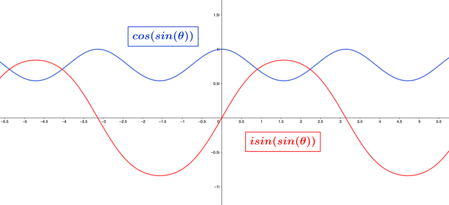
\end{array} (1.6.271) and plot each function type in the rotator submatrix in Figure 1.6.26
Figure 1.6.26 – The waveforms of the functions cos ( sin ( θ ) ) \cos\left( \sin(\theta) \right) i s i n ( sin ( θ ) ) {isin}\left( \sin(\theta) \right) The plotted waveforms above reveal the real-valued function, cos ( sin ( θ ) ) \cos\left( \sin(\theta) \right) θ \theta
cos ( sin ( π 2 + 2 π k ) ) ≈ 0.5043 , \begin{array}{r}
\cos{\left( \sin\left( \frac{\pi}{2} + 2\pi k \right) \right) \approx 0.5043},
\end{array} (1.6.272) and peaks
cos ( sin ( 2 π k ) ) = 1 , \begin{array}{r}
\cos\left( \sin(2\pi k) \right) = 1,
\end{array} (1.6.273) for k ∈ ℤ + k \in \mathbb{Z}^{+} i s i n ( sin ( θ ) ) {isin}\left( \sin(\theta) \right) θ \theta
i s i n ( sin ( 3 π 2 + 2 π k ) ) ≈ − 0.8415 , \begin{array}{r}
{isin}\left( \sin\left( \frac{3\pi}{2} + 2\pi k \right) \right) \approx - 0.8415,
\end{array} (1.6.274) and peaks
i s i n ( sin ( π 2 + 2 π k ) ) ≈ 0.8415. \begin{array}{r}
{isin}\left( \sin\left( \frac{\pi}{2} + 2\pi k \right) \right) \approx 0.8415.
\end{array} (1.6.275) Noteworthy in the plots, the waveform frequency for cos ( sin ( θ ) ) \cos\left( \sin(\theta) \right) θ = ( 0,2 π ] \theta = (0,2\pi\rbrack i s i n ( sin ( θ ) ) {isin}\left( \sin(\theta) \right) θ = ( 0,2 π ] \theta = (0,2\pi\rbrack
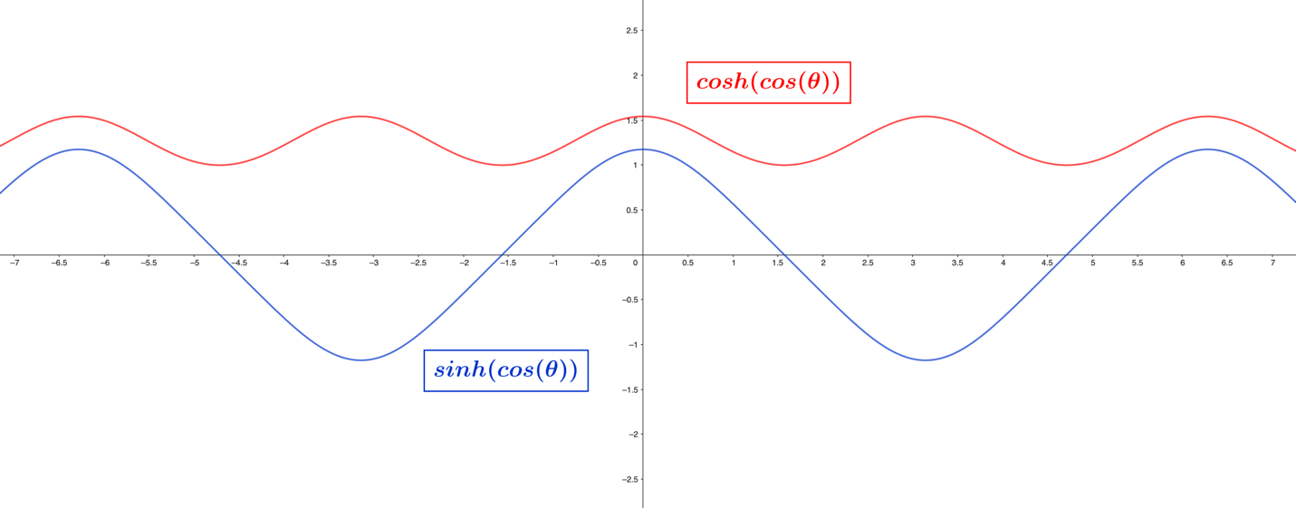
Figure 1.6.27 – Waveforms of the cosh ( cos ( θ ) ) \cosh\left( \cos(\theta) \right) sinh ( cos ( θ ) ) \sinh\left( \cos(\theta) \right) For the case of the hyperbolic group form plot, Figure 1.6.27 cosh ( cos ( θ ) ) , \cosh\left( \cos(\theta) \right), 1 1 θ \theta
cosh ( cos ( π 2 + π k ) ) = 1 , ( k ∈ ℤ + ) , \begin{array}{r}
\cosh\left( \cos\left( \frac{\pi}{2} + \pi k \right) \right) = 1,\ \ \ \left( k \in \mathbb{Z}^{+} \right),
\end{array} (1.6.276) and peaks for arguments equal to cos ( θ ) = ± 1 \cos{(\theta) = \pm 1}
cosh ( cos ( π k ) ) ≈ 1.5431 , ( k ∈ ℤ + ) , \begin{array}{r}
\cosh\left( \cos(\pi k) \right) \approx 1.5431,\ \ \ \left( k \in \mathbb{Z}^{+} \right),
\end{array} (1.6.277) The function sinh ( cos ( θ ) ) \sinh\left( \cos(\theta) \right) cosh ( cos ( θ ) ) \cosh\left( \cos(\theta) \right) θ \theta
sinh ( cos ( π + 2 π k ) ) ≈ − 1.1752 , ( k ∈ ℤ + ) \begin{array}{r}
\sinh\left( \cos(\pi + 2\pi k) \right) \approx - 1.1752,\ \ \ \left( k \in \mathbb{Z}^{+} \right)
\end{array} (1.6.278) and peaks
sinh ( cos ( 2 π k ) ) ≈ 1.1752 , ( k ∈ ℤ + ) . \begin{array}{r}
\sinh\left( \cos(2\pi k) \right) \approx 1.1752,\ \ \ \left( k \in \mathbb{Z}^{+} \right).
\end{array} (1.6.279) When considering the mathematical unit singularity, with an ontological unit radial distance from its center to its boundary, we find the complex circular functions cos ( sin ( θ ) ) \cos\left( \sin(\theta) \right) i s i n ( sin ( θ ) ) {isin}\left( \sin(\theta) \right) cosh ( cos ( θ ) ) \cosh\left( \cos(\theta) \right) sinh ( cos ( θ ) ) \sinh\left( \cos(\theta) \right) c o s − 1 ( sinh − 1 ( 1 ) ) {cos^{- 1}}\left( \sinh^{- 1}(1) \right) c o s − 1 ( sinh − 1 ( − 1 ) ) {cos^{- 1}}\left( \sinh^{- 1}( - 1) \right)
Our treatment of the Lie algebra θ r j [ D 3 𝕫 ( X 1 ) ] \theta_{r_{j}}^{\left\lbrack D_{3\mathbb{z}}\left( X_{1} \right) \right\rbrack} t j ∈ ℝ t_{j}\in \mathbb{R} t j θ r j [ D 3 𝕫 ( X 1 ) ] t_{j}\theta_{r_{j}}^{\left\lbrack D_{3\mathbb{z}}\left( X_{1} \right) \right\rbrack}
t j θ r j [ D 3 𝕫 ( X 1 ) ] = ( t 1 r 1 e i θ 1 0 0 0 0 t 2 r 2 e i θ 2 0 t 3 r 3 e i θ 3 0 ) , \begin{array}{r}
t_{j}\theta_{r_{j}}^{\left\lbrack D_{3\mathbb{z}}\left( X_{1} \right) \right\rbrack} = \begin{pmatrix}
t_{1}r_{1}e^{i\theta_{1}} & 0 & 0 \\
0 & 0 & {t_{2}r}_{2}e^{i\theta_{2}} \\
0 & {t_{3}r}_{3}e^{i\theta_{3}} & 0
\end{pmatrix},
\end{array} (1.6.280) with the complex form t j Z j [ D 3 𝕫 ( X 1 ) ] t_{j}Z_{j}^{\left\lbrack D_{3\mathbb{z}}\left( X_{1} \right) \right\rbrack}
t j Z j [ D 3 𝕫 ( X 1 ) ] = ( t 1 z 1 0 0 0 0 t 2 z 2 0 t 3 z 3 0 ) , \begin{array}{r}
t_{j}Z_{j}^{\left\lbrack D_{3\mathbb{z}}\left( X_{1} \right) \right\rbrack} = \begin{pmatrix}
t_{1}z_{1} & 0 & 0 \\
0 & 0 & t_{2}z_{2} \\
0 & t_{3}z_{3} & 0
\end{pmatrix},
\end{array} (1.6.281) and the matrix exponential mapping transforms these Lie algebras to the forms
G ( t j θ r j [ D 3 𝕫 ( X 1 ) ] ) = ( e r 1 e i θ 1 0 0 0 cosh ( t 2 r 2 t 3 r 3 e i ( θ 2 + θ 3 ) 2 ) t 2 r 2 t 3 r 3 ( e i ( θ 2 2 − θ 3 2 ) ) sinh ( t 2 r 2 t 3 r 3 e i ( θ 2 2 + θ 3 2 ) ) 0 t 3 r 3 t 2 r 2 ( e i ( θ 3 2 − θ 2 2 ) ) sinh ( r 2 r 3 e i ( θ 2 2 + θ 3 2 ) ) cosh ( t 2 r 2 t 3 r 3 e i ( θ 2 + θ 3 ) 2 ) ) , \begin{array}{r}
G\left( t_{j}\theta_{r_{j}}^{\left\lbrack D_{3\mathbb{z}}\left( X_{1} \right) \right\rbrack} \right) = \begin{pmatrix}
e^{r_{1}e^{i\theta_{1}}} & 0 & 0 \\
0 & \cosh\left( \sqrt{t_{2}r_{2}{t_{3}r}_{3}}e^{\frac{i\left( \theta_{2} + \theta_{3} \right)}{2}} \right) & \sqrt{\frac{{t_{2}r}_{2}}{t_{3}r_{3}}}\left( e^{i\left( \frac{\theta_{2}}{2} - \frac{\theta_{3}}{2} \right)} \right)\sinh\left( \sqrt{t_{2}r_{2}{t_{3}r}_{3}}e^{i\left( \frac{\theta_{2}}{2} + \frac{\theta_{3}}{2} \right)} \right) \\
0 & \sqrt{\frac{{t_{3}r}_{3}}{t_{2}r_{2}}}\left( e^{i\left( \frac{\theta_{3}}{2} - \frac{\theta_{2}}{2} \right)} \right)\sinh\left( \sqrt{r_{2}r_{3}}e^{i\left( \frac{\theta_{2}}{2} + \frac{\theta_{3}}{2} \right)} \right) & \cosh\left( \sqrt{t_{2}r_{2}{t_{3}r}_{3}}e^{\frac{i\left( \theta_{2} + \theta_{3} \right)}{2}} \right)
\end{pmatrix},
\end{array} (1.6.282) G ( t j Z j [ D 3 𝕫 ( X 1 ) ] ) = ( e t 1 z 1 0 0 0 cosh ( t 2 t 3 z 2 z 3 ) t 2 z 2 t 2 t 3 z 2 z 3 sinh ( t 2 t 3 z 2 z 3 ) 0 t 3 z 3 t 2 t 3 z 2 z 3 sinh ( t 2 t 3 z 2 z 3 ) cosh ( t 2 t 3 z 2 z 3 ) ) . \begin{array}{r}
G\left( t_{j}Z_{j}^{\left\lbrack D_{3\mathbb{z}}\left( X_{1} \right) \right\rbrack} \right) = \begin{pmatrix}
e^{t_{1}z_{1}} & 0 & 0 \\
0 & \cosh\left( \sqrt{t_{2}t_{3}z_{2}z_{3}} \right) & \frac{t_{2}z_{2}}{\sqrt{t_{2}t_{3}z_{2}z_{3}}}\sinh\left( \sqrt{t_{2}t_{3}z_{2}z_{3}} \right) \\
0 & \frac{t_{3}z_{3}}{\sqrt{t_{2}t_{3}z_{2}z_{3}}}\sinh\left( \sqrt{t_{2}t_{3}z_{2}z_{3}} \right) & \cosh\left( \sqrt{t_{2}t_{3}z_{2}z_{3}} \right)
\end{pmatrix}.
\end{array} (1.6.283) The two variables in the matrix groups above should be viewed as the means for which the subtangent space ( ln ( θ r [ m ] ) ) \left( \ln\left( \theta_{r}^{\lbrack m\rbrack} \right) \right) ( t θ r [ m ] ) \left( t\theta_{r}^{\lbrack m\rbrack} \right) ( G ( t θ r [ m ] ) ) \left( G\left( t\theta_{r}^{\lbrack m\rbrack} \right) \right) ln ( Z j [ D 3 𝕫 ( X 1 ) ] ) \ln\left( Z_{j}^{\left\lbrack D_{3\mathbb{z}}\left( X_{1} \right) \right\rbrack} \right)
ln ( Z j [ D 3 𝕫 ( X 1 ) ] ) = ( ln ( z 1 ) 0 0 0 ln ( z 2 z 3 ) + ln ( − z 2 z 3 ) 2 z 2 z 2 z 3 ( ln ( z 2 z 3 ) − ln ( − z 2 z 3 ) 2 ) 0 z 3 z 2 z 3 ( ln ( z 2 z 3 ) − ln ( − z 2 z 3 ) 2 ) ( ln ( z 2 z 3 ) + ln ( − z 2 z 3 ) ) 2 ) , \begin{array}{r}
\ln{\left( Z_{j}^{\left\lbrack D_{3\mathbb{z}}\left( X_{1} \right) \right\rbrack} \right) = \begin{pmatrix}
\ln\left( z_{1} \right) & 0 & 0 \\
0 & \frac{\ln{\left( \sqrt{z_{2}z_{3}} \right) + \ln\left( - \sqrt{z_{2}z_{3}} \right)}}{2} & \frac{z_{2}}{\sqrt{z_{2}z_{3}}}\left( \frac{\ln{\left( \sqrt{z_{2}z_{3}} \right) - \ln\left( - \sqrt{z_{2}z_{3}} \right)}}{2} \right) \\
0 & \frac{z_{3}}{\sqrt{z_{2}z_{3}}}\left( \frac{\ln{\left( \sqrt{z_{2}z_{3}} \right) - \ln\left( - \sqrt{z_{2}z_{3}} \right)}}{2} \right) & \frac{\left( \ln{\left( \sqrt{z_{2}z_{3}} \right) + \ln\left( - \sqrt{z_{2}z_{3}} \right)} \right)}{2}
\end{pmatrix}},
\end{array} (1.6.284) which using polar form variables, is
( ln ( r 1 e i θ 1 ) 0 0 0 ln ( r 2 r 3 e i ( θ 2 2 + θ 3 2 ) ) + ln ( − r 2 r 3 e i ( θ 2 2 + θ 3 2 ) ) 2 r 2 e i ( θ 2 2 − θ 3 2 ) r 2 r 3 ( ln ( r 2 r 3 e i ( θ 2 2 + θ 3 2 ) ) − ln ( − r 2 r 3 e i ( θ 2 2 + θ 3 2 ) ) 2 ) 0 r 3 e i ( θ 3 2 − θ 2 2 ) r 2 r 3 ( ln ( r 2 r 3 e i ( θ 2 2 + θ 3 2 ) ) − ln ( − r 2 r 3 e i ( θ 2 2 + θ 3 2 ) ) 2 ) ln ( r 2 r 3 e i ( θ 2 2 + θ 3 2 ) ) + ln ( − r 2 r 3 e i ( θ 2 2 + θ 3 2 ) ) 2 ) . \begin{array}{r}
\begin{pmatrix}
\ln\left( r_{1}e^{i\theta_{1}} \right) & 0 & 0 \\
0 & \frac{\ln{\left( \sqrt{r_{2}r_{3}}e^{i\left( \frac{\theta_{2}}{2} + \frac{\theta_{3}}{2} \right)} \right) + \ln\left( - \sqrt{r_{2}r_{3}}e^{i\left( \frac{\theta_{2}}{2} + \frac{\theta_{3}}{2} \right)} \right)}}{2} & \frac{r_{2}e^{i\left( \frac{\theta_{2}}{2} - \frac{\theta_{3}}{2} \right)}}{\sqrt{r_{2}r_{3}}}\left( \frac{\ln{\left( \sqrt{r_{2}r_{3}}e^{i\left( \frac{\theta_{2}}{2} + \frac{\theta_{3}}{2} \right)} \right) - \ln\left( - \sqrt{r_{2}r_{3}}e^{i\left( \frac{\theta_{2}}{2} + \frac{\theta_{3}}{2} \right)} \right)}}{2} \right) \\
0 & \frac{r_{3}e^{i\left( \frac{\theta_{3}}{2} - \frac{\theta_{2}}{2} \right)}}{\sqrt{r_{2}r_{3}}}\left( \frac{\ln{\left( \sqrt{r_{2}r_{3}}e^{i\left( \frac{\theta_{2}}{2} + \frac{\theta_{3}}{2} \right)} \right) - \ln\left( - \sqrt{r_{2}r_{3}}e^{i\left( \frac{\theta_{2}}{2} + \frac{\theta_{3}}{2} \right)} \right)}}{2} \right) & \frac{\ln{\left( \sqrt{r_{2}r_{3}}e^{i\left( \frac{\theta_{2}}{2} + \frac{\theta_{3}}{2} \right)} \right) + \ln\left( - \sqrt{r_{2}r_{3}}e^{i\left( \frac{\theta_{2}}{2} + \frac{\theta_{3}}{2} \right)} \right)}}{2}
\end{pmatrix}.
\end{array} (1.6.285) Evaluating the logarithm for each entry, the subtangent space is equivalent to
ln ( Z j [ D 3 𝕫 ( X 1 ) ] ) = ( ln ( r 1 ) + i θ 1 0 0 0 ln ( r 2 r 3 ) + i ( θ 2 + θ 3 ) + i π 2 r 2 r 3 ( e i ( θ 2 2 − θ 3 2 ) ) ( i π 2 ) 0 r 3 r 2 ( e i ( θ 3 2 − θ 2 2 ) ) ( i π 2 ) ln ( r 2 r 3 ) + i ( θ 2 + θ 3 ) + i π 2 ) , \begin{array}{r}
\ln\left( Z_{j}^{\left\lbrack D_{3\mathbb{z}}\left( X_{1} \right) \right\rbrack} \right) = \begin{pmatrix}
\ln\left( r_{1} \right) + i\theta_{1} & 0 & 0 \\
0 & \frac{\ln{\left( r_{2}r_{3} \right) + i\left( \theta_{2} + \theta_{3} \right) + i\pi}}{2} & \sqrt{\frac{r_{2}}{r_{3}}}\left( e^{i\left( \frac{\theta_{2}}{2} - \frac{\theta_{3}}{2} \right)} \right)\left( \frac{i\pi}{2} \right) \\
0 & \sqrt{\frac{r_{3}}{r_{2}}}\left( e^{i\left( \frac{\theta_{3}}{2} - \frac{\theta_{2}}{2} \right)} \right)\left( \frac{i\pi}{2} \right) & \frac{\ln{\left( r_{2}r_{3} \right) + i\left( \theta_{2} + \theta_{3} \right) + i\pi}}{2}
\end{pmatrix},
\end{array} (1.6.286) a result, with complex matrix entries, expressed in their real and imaginary portions as follows
𝓏 1 = ( 𝒶 1 + i 𝒷 1 ) = ( ln ( r 1 ) + i θ 1 ) , \begin{array}{r}
\mathcal{z}_{1} = \left( \mathcal{a}_{1} + i\mathcal{b}_{1} \right) = \left( \ln\left( r_{1} \right) + i\theta_{1} \right),
\end{array} (1.6.287) 𝓏 2 = ( 𝒶 2 + i 𝒷 2 ) = ( ( i π 2 × r 2 r 3 ) cos ( θ 2 − θ 3 2 ) + i ( i π 2 × r 2 r 3 ) sin ( θ 2 − θ 3 2 ) ) \mathcal{z}_{2} = \left( \mathcal{a}_{2} + i\mathcal{b}_{2} \right) = \left( \left( \frac{i\pi}{2} \times \sqrt{\frac{r_{2}}{r_{3}}} \right)\cos\left( \frac{\theta_{2} - \theta_{3}}{2} \right) + i\left( \frac{i\pi}{2} \times \sqrt{\frac{r_{2}}{r_{3}}} \right)\sin\left( \frac{\theta_{2} - \theta_{3}}{2} \right) \right) = ( ( π 2 × r 2 r 3 ) cos ( θ 2 − θ 3 + π 2 ) + i ( π 2 × r 2 r 3 ) sin ( θ 2 − θ 3 + π 2 ) ) , \begin{array}{r}
= \left( \left( \frac{\pi}{2} \times \sqrt{\frac{r_{2}}{r_{3}}} \right)\cos\left( \frac{\theta_{2} - \theta_{3} + \pi}{2} \right) + i\left( \frac{\pi}{2} \times \sqrt{\frac{r_{2}}{r_{3}}} \right)\sin\left( \frac{\theta_{2} - \theta_{3} + \pi}{2} \right) \right),
\end{array} (1.6.288) 𝓏 3 = ( 𝒶 3 + i 𝒷 3 ) = ( ( i π 2 × r 3 r 2 ) cos ( θ 3 − θ 2 2 ) + i ( i π 2 × r 3 r 2 ) sin ( θ 3 − θ 2 2 ) ) \mathcal{z}_{3} = \left( \mathcal{a}_{3} + i\mathcal{b}_{3} \right) = \left( \left( \frac{i\pi}{2} \times \sqrt{\frac{r_{3}}{r_{2}}} \right)\cos\left( \frac{\theta_{3} - \theta_{2}}{2} \right) + i\left( \frac{i\pi}{2} \times \sqrt{\frac{r_{3}}{r_{2}}} \right)\sin\left( \frac{\theta_{3} - \theta_{2}}{2} \right) \right) = ( ( π 2 × r 3 r 2 ) cos ( θ 3 − θ 2 + π 2 ) + i ( π 2 × r 3 r 2 ) sin ( θ 3 − θ 2 + π 2 ) ) , \begin{array}{r}
= \left( \left( \frac{\pi}{2} \times \sqrt{\frac{r_{3}}{r_{2}}} \right)\cos\left( \frac{\theta_{3} - \theta_{2} + \pi}{2} \right) + i\left( \frac{\pi}{2} \times \sqrt{\frac{r_{3}}{r_{2}}} \right)\sin\left( \frac{\theta_{3} - \theta_{2} + \pi}{2} \right) \right),
\end{array} (1.6.289) and in conjunction, the two lower entries of the main diagonal
𝓏 d = 𝓏 d = ( 𝒶 d + i 𝒷 d ) = ( ln ( r 2 r 3 ) 2 + i ( θ 2 + θ 3 + π 2 ) ) . \begin{array}{r}
\mathcal{z}_{d} = \mathcal{z}_{d} = \left( \mathcal{a}_{d} + i\mathcal{b}_{d} \right) = \left( \frac{\ln\left( r_{2}r_{3} \right)}{2} + i\left( \frac{\theta_{2} + \theta_{3} + \pi}{2} \right) \right).
\end{array} (1.6.290) With these functions in the 𝓏 j \mathcal{z}_{j} ln ( ( X 1 ( z j ) ) ) \ln\left( \left( X_{1}\left( z_{j} \right) \right) \right)
( 𝓇 1 e i Θ 1 0 0 0 𝓇 d e i Θ d 𝓇 2 e i Θ 2 0 𝓇 3 e i Θ 3 𝓇 d e i Θ d ) , \begin{array}{r}
\begin{pmatrix}
\mathcal{r}_{1}e^{i\Theta_{1}} & 0 & 0 \\
0 & \mathcal{r}_{d}e^{i\Theta_{d}} & \mathcal{r}_{2}e^{i\Theta_{2}} \\
0 & \mathcal{r}_{3}e^{i\Theta_{3}} & \mathcal{r}_{d}e^{i\Theta_{d}}
\end{pmatrix},
\end{array} (1.6.291) where each entry represents the following
𝓇 1 e i Θ 1 = 𝓏 1 = ln 2 ( r 1 ) + θ 1 2 × e i t a n − 1 ( θ 1 ln ( r 1 ) ) , \begin{array}{r}
\mathcal{r}_{1}e^{i\Theta_{1}} = \mathcal{z}_{1} = \sqrt{\ln^{2}{\left( r_{1} \right) + \theta_{1}^{2}}} \times e^{itan^{- 1}\left( \frac{\theta_{1}}{\ln\left( r_{1} \right)} \right)},
\end{array} (1.6.292) 𝓇 2 e i Θ 2 = 𝓏 2 = π 2 r 2 r 3 × e i t a n − 1 ( cot ( θ 2 − θ 3 2 ) ) , \begin{array}{r}
\mathcal{r}_{2}e^{i\Theta_{2}} = \mathcal{z}_{2} = \frac{\pi}{2}\sqrt{\frac{r_{2}}{r_{3}}} \times e^{itan^{- 1}\left( \cot\left( \frac{\theta_{2} - \theta_{3}}{2} \right) \right)},
\end{array} (1.6.293) 𝓇 3 e i Θ 3 = 𝓏 3 = π 2 r 3 r 2 × e i t a n − 1 ( cot ( θ 3 − θ 2 2 ) ) , \begin{array}{r}
\mathcal{r}_{3}e^{i\Theta_{3}} = \mathcal{z}_{3} = \frac{\pi}{2}\sqrt{\frac{r_{3}}{r_{2}}} \times e^{itan^{- 1}\left( \cot\left( \frac{\theta_{3} - \theta_{2}}{2} \right) \right)},
\end{array} (1.6.294) 𝓇 d e i Θ d = 𝓏 d = ln 2 ( r 2 r 3 ) 4 + ( θ 2 + θ 3 + π ) 2 4 × e i t a n − 1 ( θ 2 + θ 3 + π ln ( r 2 r 3 ) ) , \begin{array}{r}
\mathcal{r}_{d}e^{i\Theta_{d}} = \mathcal{z}_{d} = \sqrt{\frac{\ln^{2}\left( r_{2}r_{3} \right)}{4} + \frac{\left( \theta_{2} + \theta_{3} + \pi \right)^{2}}{4}} \times e^{itan^{- 1}\left( \frac{\theta_{2} + \theta_{3} + \pi}{\ln\left( r_{2}r_{3} \right)} \right)},
\end{array} (1.6.295) for 𝓇 j \mathcal{r}_{j} Θ j \Theta_{j} r j r_{j} θ j \theta_{j} e r e i θ e^{re^{i\theta}} r r θ \theta θ \theta G ( t j θ r j 3 , X 1 ) G\left( t_{j}\theta_{r_{j}}^{3,X_{1}} \right)
( e t 1 r 1 e i θ 1 0 0 0 cosh ( t 2 r 2 t 3 r 3 e i ( θ 2 + θ 3 ) 2 ) t 2 r 2 t 3 r 3 ( e i ( θ 2 2 − θ 3 2 ) ) sinh ( t 2 r 2 t 3 r 3 e i ( θ 2 2 + θ 3 2 ) ) 0 t 3 r 3 t 2 r 2 ( e i ( θ 3 2 − θ 2 2 ) ) sinh ( r 2 r 3 e i ( θ 2 2 + θ 3 2 ) ) cosh ( t 2 r 2 t 3 r 3 e i ( θ 2 + θ 3 ) 2 ) ) , \begin{array}{r}
\begin{pmatrix}
e^{t_{1}r_{1}e^{i\theta_{1}}} & 0 & 0 \\
0 & \cosh\left( \sqrt{t_{2}r_{2}{t_{3}r}_{3}}e^{\frac{i\left( \theta_{2} + \theta_{3} \right)}{2}} \right) & \sqrt{\frac{{t_{2}r}_{2}}{t_{3}r_{3}}}\left( e^{i\left( \frac{\theta_{2}}{2} - \frac{\theta_{3}}{2} \right)} \right)\sinh\left( \sqrt{t_{2}r_{2}{t_{3}r}_{3}}e^{i\left( \frac{\theta_{2}}{2} + \frac{\theta_{3}}{2} \right)} \right) \\
0 & \sqrt{\frac{{t_{3}r}_{3}}{t_{2}r_{2}}}\left( e^{i\left( \frac{\theta_{3}}{2} - \frac{\theta_{2}}{2} \right)} \right)\sinh\left( \sqrt{r_{2}r_{3}}e^{i\left( \frac{\theta_{2}}{2} + \frac{\theta_{3}}{2} \right)} \right) & \cosh\left( \sqrt{t_{2}r_{2}{t_{3}r}_{3}}e^{\frac{i\left( \theta_{2} + \theta_{3} \right)}{2}} \right)
\end{pmatrix},
\end{array} (1.6.296) and consider this group for all r j = 1 , r_{j} = 1, θ j = π 2 \theta_{j} = \frac{\pi}{2} G ( t j θ ( π 2 ) 1 [ D 3 𝕫 ( X 1 ) ] ) G\left( t_{j}{\theta\left( \frac{\pi}{2} \right)}_{1}^{\left\lbrack D_{3\mathbb{z}}\left( X_{1} \right) \right\rbrack} \right)
G ( t j θ ( π 2 ) 1 [ D 3 𝕫 ( X 1 ) ] ) = ( e t 1 e i π 2 0 0 0 cosh ( t 2 t 3 e i π 2 ) t 2 t 3 sinh ( t 2 t 3 e i π 2 ) 0 t 3 t 2 sinh ( t 2 t 3 e i π 2 ) cosh ( t 2 t 3 e i π 2 ) ) . \begin{array}{r}
G\left( t_{j}{\theta\left( \frac{\pi}{2} \right)}_{1}^{\left\lbrack D_{3\mathbb{z}}\left( X_{1} \right) \right\rbrack} \right) = \begin{pmatrix}
e^{t_{1}e^{\frac{i\pi}{2}}} & 0 & 0 \\
0 & \cosh\left( \sqrt{t_{2}t_{3}}e^{\frac{i\pi}{2}} \right) & \sqrt{\frac{t_{2}}{t_{3}}}\sinh\left( \sqrt{t_{2}t_{3}}e^{\frac{i\pi}{2}} \right) \\
0 & \sqrt{\frac{t_{3}}{t_{2}}}\sinh\left( \sqrt{t_{2}t_{3}}e^{\frac{i\pi}{2}} \right) & \cosh\left( \sqrt{t_{2}t_{3}}e^{\frac{i\pi}{2}} \right)
\end{pmatrix}.
\end{array} (1.6.297) The example for the chosen variables, results in a e ( i π 2 ) \ e^{\left( \frac{i\pi}{2} \right)}
G ( t j θ ( π 2 ) 1 [ D 3 𝕫 ( X 1 ) ] ) = ( e i t 1 0 0 0 cosh ( i t 2 t 3 ) t 2 t 3 sinh ( i t 2 t 3 ) 0 t 3 t 2 sinh ( i t 2 t 3 ) cosh ( i t 2 t 3 ) ) , \begin{array}{r}
G\left( t_{j}{\theta\left( \frac{\pi}{2} \right)}_{1}^{\left\lbrack D_{3\mathbb{z}}\left( X_{1} \right) \right\rbrack} \right) = \begin{pmatrix}
e^{it_{1}} & 0 & 0 \\
0 & \cosh\left( i\sqrt{t_{2}t_{3}} \right) & \sqrt{\frac{t_{2}}{t_{3}}}\sinh\left( i\sqrt{t_{2}t_{3}} \right) \\
0 & \sqrt{\frac{t_{3}}{t_{2}}}\sinh\left( i\sqrt{t_{2}t_{3}} \right) & \cosh\left( i\sqrt{t_{2}t_{3}} \right)
\end{pmatrix},
\end{array} (1.6.298) and given the identities, sinh ( i θ ) = i s i n ( θ ) , cosh ( i θ ) = cos ( θ ) , \sinh{(i\theta) = isin(\theta),}\cosh{(i\theta) = \cos(\theta),} G ( t j θ ( π 2 ) 1 [ D 3 𝕫 ( X 1 ) ] ) G\left( t_{j}{\theta\left( \frac{\pi}{2} \right)}_{1}^{\left\lbrack D_{3\mathbb{z}}\left( X_{1} \right) \right\rbrack} \right)
G ( t j θ ( π 2 ) 1 [ D 3 𝕫 ( X 1 ) ] ) = ( e i t 1 0 0 0 cos ( t 2 t 3 ) t 2 t 3 × i s i n ( t 2 t 3 ) 0 t 3 t 2 × i s i n ( t 2 t 3 ) cos ( t 2 t 3 ) ) . \begin{array}{r}
G\left( t_{j}{\theta\left( \frac{\pi}{2} \right)}_{1}^{\left\lbrack D_{3\mathbb{z}}\left( X_{1} \right) \right\rbrack} \right) = \begin{pmatrix}
e^{it_{1}} & 0 & 0 \\
0 & \cos\left( \sqrt{t_{2}t_{3}} \right) & \sqrt{\frac{t_{2}}{t_{3}}}{\times isin}\left( \sqrt{t_{2}t_{3}} \right) \\
0 & \sqrt{\frac{t_{3}}{t_{2}}}{\times isin}\left( \sqrt{t_{2}t_{3}} \right) & \cos\left( \sqrt{t_{2}t_{3}} \right)
\end{pmatrix}.
\end{array} (1.6.299) By assuming the t j t_{j} G ( t θ ( π 2 ) 1 [ D 3 𝕫 ( X 1 ) ] ) G\left( t{\theta\left( \frac{\pi}{2} \right)}_{1}^{\left\lbrack D_{3\mathbb{z}}\left( X_{1} \right) \right\rbrack} \right) U ( 3 ) U(3) G ( i X 1 ) G\left( iX_{1} \right)
G ( t θ ( π 2 ) 1 [ D 3 𝕫 ( X 1 ) ] ) = G ( i X 1 ) = ( e i t 0 0 0 cos ( t ) i s i n ( t ) 0 i s i n ( t ) cos ( t ) ) . \begin{array}{r}
G\left( t{\theta\left( \frac{\pi}{2} \right)}_{1}^{\left\lbrack D_{3\mathbb{z}}\left( X_{1} \right) \right\rbrack} \right) = G\left( iX_{1} \right) = \begin{pmatrix}
e^{it} & 0 & 0 \\
0 & \cos(t) & {isin}(t) \\
0 & {isin}(t) & \cos(t)
\end{pmatrix}.
\end{array} (1.6.300) Angle space rotations that occur on the singularity's boundary can be represented in multiple ways, shown first, by using the X 1 X_{1}
θ r j [ D 3 𝕫 ( X 1 ) ] × ( θ r j [ D 3 𝕫 ( X 1 ) ] ) T × X 1 = ( 2 θ ) r 2 [ D 3 𝕫 ( X 1 ) ] \theta_{r_{j}}^{\left\lbrack D_{3\mathbb{z}}\left( X_{1} \right) \right\rbrack} \times \left( \theta_{r_{j}}^{\left\lbrack D_{3\mathbb{z}}\left( X_{1} \right) \right\rbrack} \right)^{T} \times X_{1} = (2\theta)_{r^{2}}^{\left\lbrack D_{3\mathbb{z}}\left( X_{1} \right) \right\rbrack} = ( r 1 e i θ 1 0 0 0 0 r 2 e i θ 2 0 r 3 e i θ 3 0 ) ( r 1 e i θ 1 0 0 0 0 r 3 e i θ 3 0 r 2 e i θ 2 0 ) ( 1 0 0 0 0 1 0 1 0 ) = ( r 1 2 e i 2 θ 1 0 0 0 0 r 2 2 e i 2 θ 2 0 r 3 2 e i 2 θ 3 0 ) , \begin{array}{r}
= \begin{pmatrix}
r_{1}e^{i\theta_{1}} & 0 & 0 \\
0 & 0 & r_{2}e^{i\theta_{2}} \\
0 & r_{3}e^{i\theta_{3}} & 0
\end{pmatrix}\begin{pmatrix}
r_{1}e^{i\theta_{1}} & 0 & 0 \\
0 & 0 & r_{3}e^{i\theta_{3}} \\
0 & r_{2}e^{i\theta_{2}} & 0
\end{pmatrix}\begin{pmatrix}
1 & 0 & 0 \\
0 & 0 & 1 \\
0 & 1 & 0
\end{pmatrix} = \begin{pmatrix}
r_{1}^{2}e^{i{2\theta}_{1}} & 0 & 0 \\
0 & 0 & r_{2}^{2}e^{i{2\theta}_{2}} \\
0 & r_{3}^{2}e^{i2\theta_{3}} & 0
\end{pmatrix},
\end{array} (1.6.301) which serves to rotate each polar variable in the Lie algebra θ r j [ D 3 𝕫 ( X 1 ) ] \theta_{r_{j}}^{\left\lbrack D_{3\mathbb{z}}\left( X_{1} \right) \right\rbrack} v ˆ = ( e i ρ 1 , e i ρ 2 , e i ρ 3 ) \widehat{v} = \left( e^{i\rho_{1}},e^{i\rho_{2}},e^{i\rho_{3}} \right) ρ j ∈ ℝ \rho_{j}\in \mathbb{R} θ r j [ D 3 𝕫 ( X 1 ) ] \theta_{r_{j}}^{\left\lbrack D_{3\mathbb{z}}\left( X_{1} \right) \right\rbrack}
d i a g ( v ˆ ) × θ r j [ D 3 𝕫 ( X 1 ) ] = ( ρ + θ ) r j [ D 3 𝕫 ( X 1 ) ] diag\left( \widehat{v} \right) \times \theta_{r_{j}}^{\left\lbrack D_{3\mathbb{z}}\left( X_{1} \right) \right\rbrack} = (\rho + \theta)_{r_{j}}^{\left\lbrack D_{3\mathbb{z}}\left( X_{1} \right) \right\rbrack} = ( e i ρ 1 0 0 0 e i ρ 2 0 0 0 e i ρ 3 ) ( r 1 e i θ 1 0 0 0 0 r 2 e i θ 2 0 r 3 e i θ 3 0 ) = ( r 1 e i ( θ 1 + ρ 1 ) 0 0 0 0 r 2 e i ( θ 2 + ρ 2 ) 0 r 3 e i ( θ 3 + ρ 3 ) 0 ) . \begin{array}{r}
= \begin{pmatrix}
e^{i\rho_{1}} & 0 & 0 \\
0 & e^{i\rho_{2}} & 0 \\
0 & 0 & e^{i\rho_{3}}
\end{pmatrix}\begin{pmatrix}
r_{1}e^{i\theta_{1}} & 0 & 0 \\
0 & 0 & r_{2}e^{i\theta_{2}} \\
0 & r_{3}e^{i\theta_{3}} & 0
\end{pmatrix} = \begin{pmatrix}
r_{1}e^{i\left( \theta_{1} + \rho_{1} \right)} & 0 & 0 \\
0 & 0 & r_{2}e^{i\left( \theta_{2} + \rho_{2} \right)} \\
0 & r_{3}e^{i\left( \theta_{3} + \rho_{3} \right)} & 0
\end{pmatrix}.
\end{array} (1.6.302) To gain further intuition on how a rotation in the angle space affects geometry, we set θ j = π 2 , r j = r , \theta_{j} = \frac{\pi}{2},\ r_{j} = r, v ˆ = ( e ( − i π 2 ) , e ( − i π 2 ) , e ( − i π 2 ) ) , \widehat{v} = \left( e^{\left( - \frac{i\pi}{2} \right)},e^{\left( - \frac{i\pi}{2} \right)},e^{\left( - \frac{i\pi}{2} \right)} \right),
d i a g ( v ˆ ) × θ r [ i × | D 3 𝕫 ( X 1 ) | ] = ( − π 2 + π 2 ) r [ D 3 𝕫 ( X 1 ) ] = θ r [ | D 3 𝕫 ( X 1 ) | ] diag\left( \widehat{v} \right) \times \theta_{r}^{\left\lbrack {i \times |D}_{3\mathbb{z}}\left( X_{1} \right)| \right\rbrack} = \left( - \frac{\pi}{2} + \frac{\pi}{2} \right)_{r}^{\left\lbrack D_{3\mathbb{z}}\left( X_{1} \right) \right\rbrack} = \theta_{r}^{\left\lbrack {|D}_{3\mathbb{z}}\left( X_{1} \right)| \right\rbrack} = ( e − i π 2 0 0 0 e − i π 2 0 0 0 e − i π 2 ) ( i r 0 0 0 0 i r 0 i r 0 ) = ( r 0 0 0 0 r 0 r 0 ) , \begin{array}{r}
= \begin{pmatrix}
e^{- \frac{i\pi}{2}} & 0 & 0 \\
0 & e^{- \frac{i\pi}{2}} & 0 \\
0 & 0 & e^{- \frac{i\pi}{2}}
\end{pmatrix}\begin{pmatrix}
ir & 0 & 0 \\
0 & 0 & ir \\
0 & ir & 0
\end{pmatrix} = \begin{pmatrix}
r & 0 & 0 \\
0 & 0 & r \\
0 & r & 0
\end{pmatrix},
\end{array} (1.6.303) finding the rotation in the angle space has changed the geometry from the imaginary-valued X 1 X_{1} i × | D 3 𝕫 | {i \times |D}_{3\mathbb{z}}| X 1 X_{1} | D 3 𝕫 | |D_{3\mathbb{z}}|
The content of this chapter, and in particular this section, leads to the following definition of The Tangent Space Complex Symmetry Group .
Definition (1.6.304) – We define The Tangent Space Complex Symmetry Group 𝛉 𝐫 𝐣 [ 𝐃 𝟑 𝕫 ( 𝐗 𝐤 , 𝐘 𝐤 ) ] ∈ ℂ 3 \mathbf{\theta}_{\mathbf{r}_{\mathbf{j}}}^{\left\lbrack \mathbf{D}_{\mathbf{3}\mathbb{z}}\left( \mathbf{X}_{\mathbf{k}}\mathbf{,}\mathbf{Y}_{\mathbf{k}} \right) \right\rbrack} \in \mathbb{C}^{3} , as a group under composition, comprised of C ∞ C^{\infty} functions for its infinitesimal minimal element basis ∈ ℂ 3 , \in \mathbb{C}^{3}, yielding the infinite set θ r [ m ] ∞ {\theta_{r}^{\lbrack m\rbrack}}^{\infty} of unitary elements in tangent space, for r j r_{j} =1, and non-unit radial lengths r j ≠ 1 r_{j} \neq 1 , for the form extended or contracted in ℂ 3 \mathbb{C}^{3} -space from the unitary state
θ r j [ D 3 𝕫 ( X k , Y k ) ] = { θ r [ m ] ∞ ∈ G L ( 3 , ℂ ) | θ r [ m ] ∞ ∙ ( θ r [ m ] ∞ ) † = 𝓇 2 I } , \begin{array}{r}
\theta_{r_{j}}^{\left\lbrack D_{3\mathbb{z}}\left( X_{k},Y_{k} \right) \right\rbrack}\ = \left\{ {\theta_{r}^{\lbrack m\rbrack}}^{\infty} \in GL\left( 3,\mathbb{C} \right)|{\theta_{r}^{\lbrack m\rbrack}}^{\infty} \bullet \left( {\theta_{r}^{\lbrack m\rbrack}}^{\infty} \right)^{\dagger} = \mathcal{r}^{2}I\ \right\},
\end{array} containing element sets,
θ r j [ D 3 𝕫 ( X k ) ] = { ( r 1 e i θ ( 1,1 ) 0 0 0 0 r 2 e i θ ( 1,2 ) 0 r 3 e i θ ( 1,3 ) 0 ) , ( 0 0 r 1 e i θ ( 2,1 ) 0 r 2 e i θ ( 2,2 ) 0 r 3 e i θ ( 2,3 ) 0 0 ) , ( 0 r 1 e i θ ( 3,1 ) 0 r 2 e i θ ( 3,2 ) 0 0 0 0 r 3 e i θ ( 3,3 ) ) } , \theta_{r_{j}}^{\left\lbrack D_{3\mathbb{z}}\left( X_{k} \right) \right\rbrack} = \left\{ \begin{array}{r}
\begin{pmatrix}
r_{1}e^{i\theta_{(1,1)}} & 0 & 0 \\
0 & 0 & r_{2}e^{i\theta_{(1,2)}} \\
0 & r_{3}e^{i\theta_{(1,3)}} & 0
\end{pmatrix},\begin{pmatrix}
0 & 0 & r_{1}e^{i\theta_{(2,1)}} \\
0 & r_{2}e^{i\theta_{(2,2)}} & 0 \\
r_{3}e^{i\theta_{(2,3)}} & 0 & 0
\end{pmatrix}, \\
\begin{pmatrix}
0 & r_{1}e^{i\theta_{(3,1)}} & 0 \\
r_{2}e^{i\theta_{(3,2)}} & 0 & 0 \\
0 & 0 & r_{3}e^{i\theta_{(3,3)}}
\end{pmatrix}
\end{array} \right\}, θ r ( k , j ) [ D 3 𝕫 ( Y k ) ] = { ( r 1 e i θ ( 1,1 ) 0 0 0 0 r 2 e i θ ( 1,2 ) 0 r 3 e i θ ( 1,3 ) 0 ) , ( 0 0 r 1 e i θ ( 2,1 ) 0 r 2 e i θ ( 2,2 ) 0 r 3 e i θ ( 2,3 ) 0 0 ) , ( 0 r 1 e i θ ( 3,1 ) 0 r 2 e i θ ( 3,2 ) 0 0 0 0 r 3 e i θ ( 3,3 ) ) } . \theta_{r_{(k,j)}}^{\left\lbrack D_{3\mathbb{z}}\left( Y_{k} \right) \right\rbrack} = \left\{ \begin{array}{r}
\begin{pmatrix}
r_{1}e^{i\theta_{(1,1)}} & 0 & 0 \\
0 & 0 & r_{2}e^{i\theta_{(1,2)}} \\
0 & r_{3}e^{i\theta_{(1,3)}} & 0
\end{pmatrix},\begin{pmatrix}
0 & 0 & r_{1}e^{i\theta_{(2,1)}} \\
0 & r_{2}e^{i\theta_{(2,2)}} & 0 \\
r_{3}e^{i\theta_{(2,3)}} & 0 & 0
\end{pmatrix}, \\
\begin{pmatrix}
0 & r_{1}e^{i\theta_{(3,1)}} & 0 \\
r_{2}e^{i\theta_{(3,2)}} & 0 & 0 \\
0 & 0 & r_{3}e^{i\theta_{(3,3)}}
\end{pmatrix}
\end{array} \right\}. Theorem (1.6.305) –For θ r [ m ] ∞ {\theta_{r}^{\lbrack m\rbrack}}^{\infty} as a set, the set of permutations θ r j [ D 3 𝕫 ( X k , Y k ) ] \theta_{r_{j}}^{\left\lbrack D_{3\mathbb{z}}\left( X_{k},Y_{k} \right) \right\rbrack} forms a group under composition.
Proof – Verification of group axioms
Closure: All elements ∈ θ r [ m ] ∞ \in {\theta_{r}^{\lbrack m\rbrack}}^{\infty} are bijective, and the composition of elements ϕ ∘ ψ ∈ θ r [ m ] ∞ \phi \circ \psi\ \in {\theta_{r}^{\lbrack m\rbrack}}^{\infty} is also bijective.
Associativity: Permutations are functions, and their compositions are associative.
Identity: The identity function ϵ ( Y 1 ) \epsilon_{\left( Y_{1} \right)} bijectively maps all elements in the set θ r [ m ] ∞ {\theta_{r}^{\lbrack m\rbrack}}^{\infty} to themselves ( ϵ ( Y 1 ) : θ r [ m ] ∞ → θ r [ m ] ∞ ) \left( \epsilon_{\left( Y_{1} \right)}:{\theta_{r}^{\lbrack m\rbrack}}^{\infty} \rightarrow {\theta_{r}^{\lbrack m\rbrack}}^{\infty} \right) .
Inverse: ϕ \phi is a permutation and is thus bijective, and there exists a function ϕ − 1 \phi^{- 1} that is also bijective.
□ \square