1.4.1 Matrix Group Conic Sections

Our stud­ies of matrix groups stem­ming from the di­he­dral forms in com­plex geo­met­ric spaces lend them­selves to fur­ther clas­si­fi­ca­tion and group­ing in a com­plex conic space. The analy­sis of conic sec­tions has been around since an­tiq­ui­ty and in­volves cut­ting cones with a plane to obtain curves. The conics sec­tions are typ­i­cal­ly taught to be the in­ter­sec­tions of planes that do not pass through the cone's origin. Each plane can meet the cone in three ways to create in­ter­sect­ing curves: the parabo­la, the el­lipse, and the hy­per­bo­la, as seen in Figure 1.4.1 below.

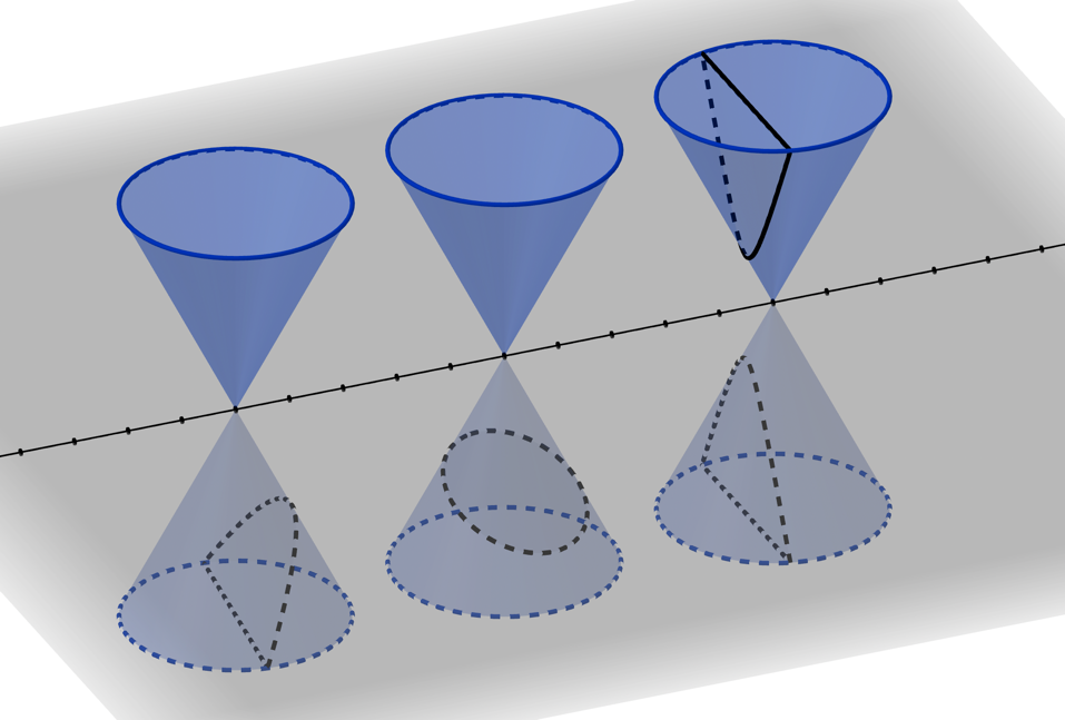
For real-valued-based conic sec­tions, if a plane aligned with the $z$-axis passed through the origin, a null curve would be the result, which is simply the two lines that form the bound­ary of the cone. When con­sid­er­ing a cone ori­ent­ed length­wise along the z-axis, the equa­tion of this cone $\in \mathbb{R}^{3}$ can be rep­re­sent­ed as

where $k$ is a con­stant.¹ For the value of $x = 0$, the above equa­tion of the cone will become

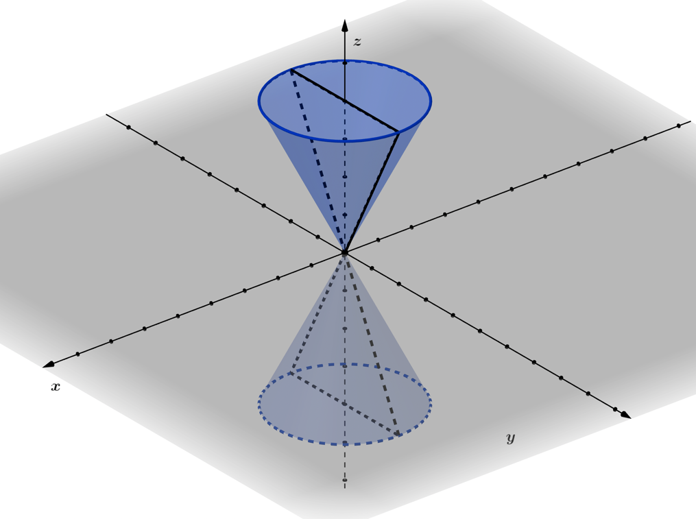
and this is simply the equa­tion of two lines, which is the null curve as seen in Figure 1.4.2. To con­sid­er the al­ge­bra­ic dif­fer­ences be­tween the parabo­la, el­lipse, and hy­per­bo­la, we take the cone to be sym­met­ric about the z-axis, as­sum­ing a cut­ting plane which is per­pen­dic­u­lar to the $y,z$-plane, having the equa­tion

Di­vid­ing by the co­ef­fi­cient for $z$, or by the co­ef­fi­cient for $y,$and by set­ting for each the re­spec­tive $y,z = 0$, yields the fol­low­ing cut­ting planes

Let $f/c = e$. For the cut­ting plane, when $y = e,$the plane can move up and down along the $y$-axis only as $z = 0$, and hy­per­bol­ic curves result, except for the null curve when $y = 0.$Sub­sti­tut­ing this into our equa­tion of the cone, we find

which is the re­sult­ing hy­per­bo­la. For $z \neq 0$, we can solve $cy + z = e$ for $z$, find­ing, $z = e - cy$, which we insert into our orig­i­nal equa­tion of the cone to find

It is im­por­tant to note that the co­ef­fi­cient of $y^{2}$ will depend on the slope of $- c$, for the cut­ting plane, and the fol­low­ing re­la­tion­ships hold for that slope

• Less than 0 for $c^{2} > k^{2}$ - occurs for conics that are hy­per­bo­lae.

• Greater than 0 for $c^{2} < k^{2}$ - occurs for conics that are el­lipses.

• Equal to 0 for $c^{2} = k^{2}$ - occurs for conics that are parabo­la.

The equa­tion $x^{2} + y^{2}\left( 1 - k^{2}c^{2} \right) + 2k^{2}ecy = k^{2}e^{2}$ rep­re­sents the re­la­tion­ship be­tween $x$ and $y$ on the conic sec­tion and is the curve's pro­jec­tion in the $x,y$-plane. Taking, $\left( 1 - k^{2}c^{2} \right)$, as equal to zero or not, we can sim­pli­fy the equa­tion as

where, $D = 2k^{2}ec$, $C = ke$, $A = \left( 1 - k^{2}c^{2} \right),\ B = \frac{k^{2}ec}{1 - k^{2}c^{2}}.$Next, by re­plac­ing $y = \left( y - \frac{C^{2}}{D} \right)$, for $x^{2} = Dy + C^{2}$, and $y = (y + B)$, for $\ x^{2} + A{(y}^{2} + 2By) = C^{2}$, the above become

For $x^{2} = Dy$, we divide both sides by $D$, set, $\frac{1}{D} = a$, and find the fa­mil­iar equa­tion of the parabo­la

For $x^{2} + Ay^{2} = C^{2} - AB^{2}$, mul­ti­ply­ing by $1/A$, and di­vid­ing by $\left( \frac{C^{2}}{A} - B^{2} \right)$, yields

and by sub­sti­tut­ing $a^{2} = \left( C^{2} - \frac{B^{2}}{A} \right),\ b^{2} = \left( \frac{C^{2}}{A} - B^{2} \right)$, for $\frac{C^{2}}{A} > B^{2}$, and $- b^{2} = \left( \frac{C^{2}}{A} - B^{2} \right)$, for $\frac{C^{2}}{A} < B^{2}$, we have equa­tions for the el­lipse

and the hy­per­bo­la

As we con­tin­ue, we will find the "null curve", rep­re­sent­ing the side of the cone in com­plex space, plays a piv­otal role math­e­mat­i­cal­ly in con­trast to the real conics, the in­ter­sec­tion of the top and bottom points of cones is not a zero-di­men­sion­al point but in­stead our $U(3)$ sphere, and we ap­proach these conics by using the frame­works of tan­gent spaces and com­plex-valued angles.

1. Still­well, John– "Num­bers and Geom­e­try", Springer, 2000