This book focuses on the equilateral triangle's group representation as our regular polygon form space. Higher-dimensional forms exist that are simple to define given the work we have already done with the symmetry group. In the process of considering these forms, we find the associations that are inherent to odd and even-numbered vertex sets of the regular polygon. This will have future implications related to the Poincaré-Hopf theorem, which states that there are no smooth vector fields on an even-dimensional -sphere without sources or sinks.
Before proceeding, we consider the eigenvalues for the Lie algebra generators
(1.7.159)
which have in diagonalized eigenvalue matrices
(1.7.160)
We recall the primary generators of the set are
(1.7.161)
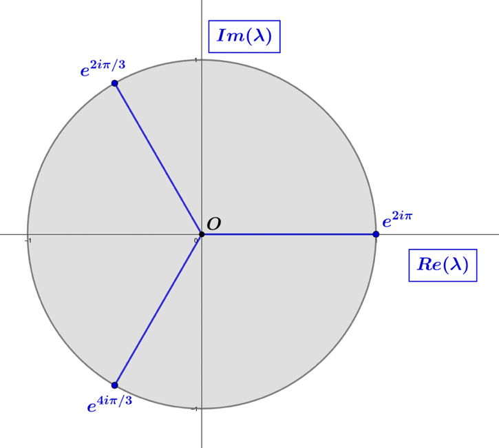
finding these Lie algebras have complex eigenvalues equal to the values of the vertices of the inscribed equilateral triangle in the complex unit circle.
The fundamental theory of algebra states that at least one complex root exists for every single variable and non-constant polynomial having complex coefficients. Given that real coefficients are complex numbers with imaginary portions equal to zero, the theory also includes polynomials with real coefficients. When the fundamental theory of algebra is applied to an matrix and its characteristic polynomial of degree , it implies that this polynomial can be factored into a product of linear terms.
For clarity in regard to applying the fundamental theory of algebra with matrix theory, we take a closer look at calculating the eigenvalues for the matrix . We start by setting to equal zero
(1.7.162)
and it is apparent that for the eigenvalues of the matrix to exist, the determinant of the matrix must be zero. The characteristic polynomial of is found by calculating the determinant of
(1.7.163)
We substitute this polynomial result back into the initial expression
(1.7.164)
and after solving for , we find
(1.7.165)
which has the three solutions in complex space . Having the eigenvalue solutions of the characteristic polynomial, and by the implications of the fundamental theory of algebra, we can express the polynomial as the following product of linear terms
(1.7.166)
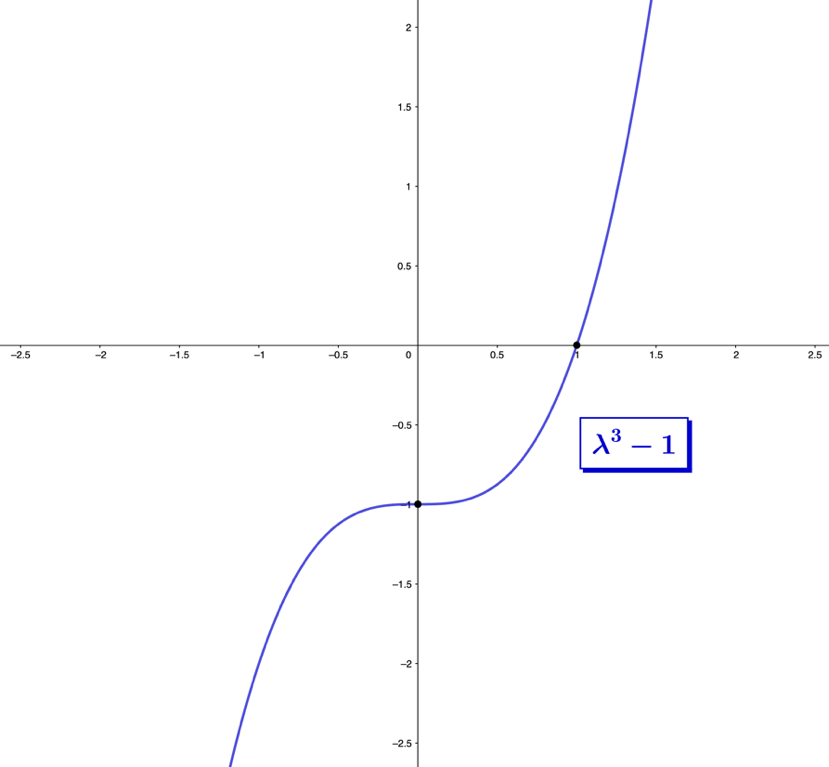
We plot this product of linear terms in the figure below, for which the function crosses the -axis at when , having roots at the point on the graph when the function crosses the -axis at .
Figure 1.7.11 – Plot of the characteristic polynomial function
with roots equal to the eigenvalues of the matrix.
In Figure 1.7.11, the roots in the complex plane have the same arrangement as the inscribed equilateral triangle defined as the geometric prime in the last section. In contrast, the matrix generators' eigenvalues, which comprise the set
(1.7.167)
are all real-valued, with characteristic polynomials of the form
(1.7.168)
and the solutions to the equation
(1.7.169)
represent the eigenvalues of the set of matrices, .
Figure 1.7.12 – The roots in complex space of polynomial
which are equal to the eigenvalues of the matrix.
As previously discussed, these Lie algebra generators will take on complex values, and for any matrix defined as the product , for , its eigenvalues will equal
(1.7.170)
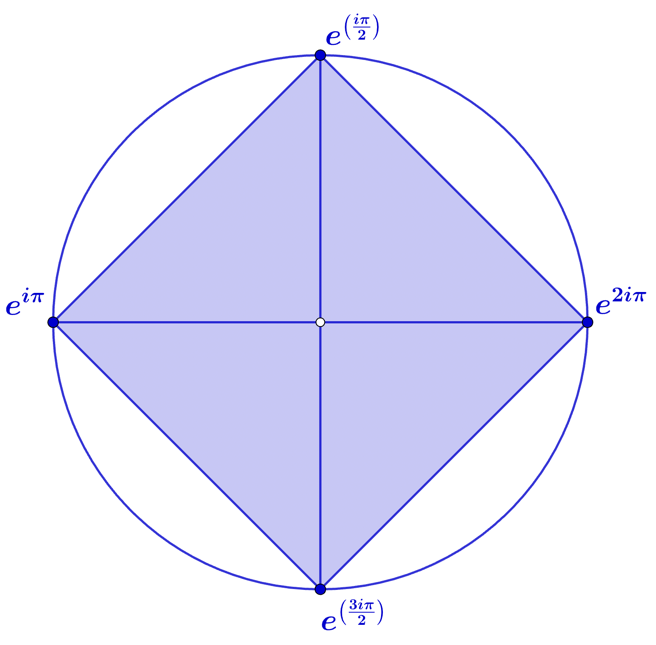
We continue to consider the higher-dimensional forms by first looking at the inscribed square in Figure 1.7.13, which, like the equilateral triangle, can be rotated uniformly in the complex plane, representing an orderly cyclic shifting of the vertices.
Figure 1.7.13 – The inscribed regular square polygon in the complex unit circle.
It is important to note that this cyclic shift of the vertices occurs in a single complex plane. In a similar manner to previous cyclic permutation matrices, the set of matrices are
(1.7.171)
but what differs with the matrices, , is that the third matrix in the set, , like the identity, is not capable of generating all the permutation elements of the set. This can be seen by taking odd and even integer powers of the matrix
(1.7.172)
(1.7.173)
which results in either the identity matrix, , or itself. The reason behind this is that the matrix shifts all vertices by two locations and given that the four vertices of the square are an even number, only half of the cyclic rotations are possible. What stands out about the matrix is that, like the identity matrix, it is symmetric about both the main diagonal and the anti-diagonal, and this differs from the lone symmetry have about the anti-diagonal.
The matrix-vector product representation of the cyclic rotation of vertices by the matrix is
(1.7.174)
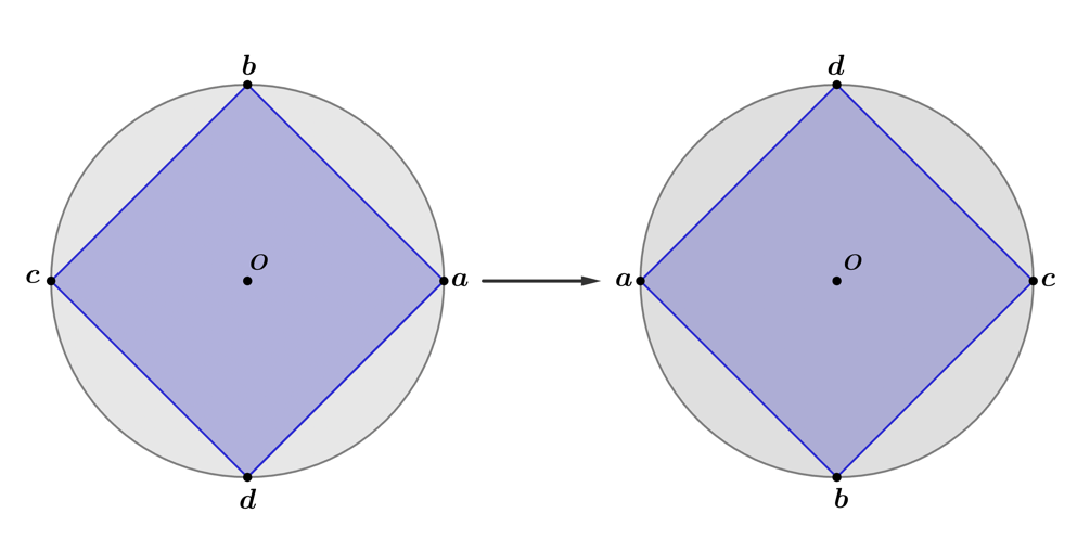
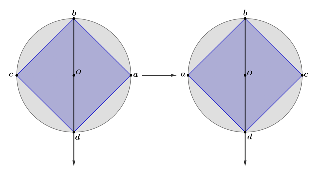
for which, the vector entries represent the vertices of the regular square polygon. Graphically, we represent this cyclic rotation in the complex plane below, where the left square has its vertices positioned as , and the matrix-vector product transforms the positions of the vertices to that found in the right square. The primary generators of the set are the subset
(1.7.175)
Figure 1.7.14 – The cyclic rotation
These have the following characteristic polynomials
(1.7.176)
which is like the characteristic polynomial, , of the primary generators . Solving the characteristic polynomial expression
(1.7.177)
we also find eigenvalue solutions, , aligned with the distinct vertex values of the inscribed sphere on the complex unit circle. In contrast to the primary generators, the characteristic polynomials of the other Lie algebras in the set are found to be
(1.7.178)
(1.7.179)
whose eigenvalues are solutions to the equations
(1.7.180)
(1.7.181)
which are real-valued and not entirely distinct.
To find the Lie algebra generators that are responsible for the higher-dimensional rotations around the axes of the square partitioning it into equal sections, we define the anti-identity for the group as
(1.7.182)
and calculate the matrix-matrix product set
(1.7.183)
The products involve the Lie algebra generators that had dual symmetry along the matrix diagonal and anti-diagonal, and these also yield Lie algebra generators in the set , characterized by this dual symmetry, . The commutator of the matrices and is equal to zero, given the dual symmetry they have in common
(1.7.184)
and we can further classify both matrices as symmetric, meaning the transpose of each matrix is equal to itself. We also find that the commutator of the matrices and is equal to zero
(1.7.185)
since the transpose matrix of each is equal to the matrix itself
(1.7.186)
Given that both are orthogonal matrices, the following holds
(1.7.187)
(1.7.188)
Continuing, we find the following relationship with the commutators
(1.7.189)
(1.7.190)
The set of rotation matrices flips the square by two distinct axes, the first along axes that are vertex-to-vertex oriented, and the second axis is formed by the equally partitioning of two opposite polygon edges. The and rotation matrices flip vertices around a vertex-to-vertex oriented axis, where the matrix-vector products are
(1.7.191)
(1.7.192)
So, the entries along the main diagonals of and act to leave the coinciding vertex position unchanged, while non-diagonal entries work to flip the vertex positions. Graphically we depict the matrix-vector product in the following figure, where the axis of rotation is described as the vector, and we see that the vertices and remain unchanged, while the and vertices have exchanged positions.
Figure 1.7.15 – The matrix-vector product and its -axis of rotation.
In contrast, the and rotation matrices flip vertices around an edge-to-edge oriented axis, where the matrix-vector products are
(1.7.193)
(1.7.194)
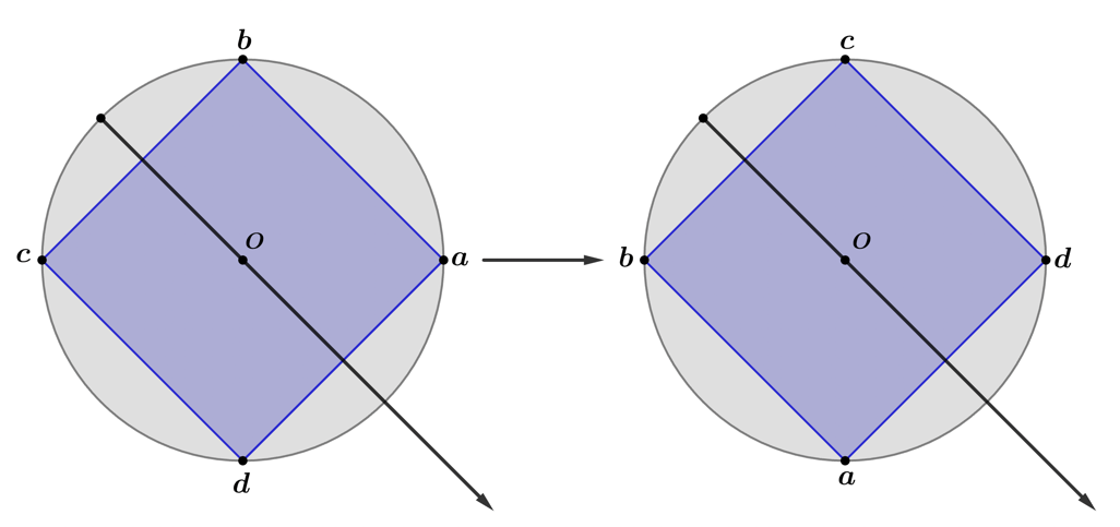
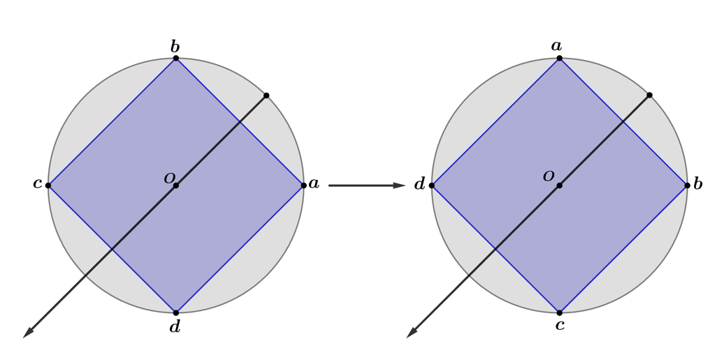
which leads to all vertices moving position, given that neither matrix has entries on the diagonal. The next two figures graphically depict both rotations, with the axis of rotation for the rotation being , and that of rotation being
Figure 1.7.16 – The matrix-vector product and its -axis of rotation.
Figure 1.7.17– The matrix-vector product and its -axis of rotation.
At this juncture, it is essential to point out that the set of generators for the inscribed -gons represent complex numbers, and the eigenvalues of each generator represent the vertices that each number will inscribe on the boundary of the unit circle. For the set , when is non-prime, the set of generators will be composite in terms of the numbers they represent. In the case for the set , the Lie algebra generator is
(1.7.195)
whose set of eigenvalues is , and the generator represents the minimal element in either the positive or negative rotational orientation, . There are two possible numbers that may represent; or , since both numbers are primary generators since they can generate all the eigenvalues in the set , given that
(1.7.196)
For clarity, we will define as the first cyclic shift of the identity rightward
(1.7.197)
and we define as the first cyclic shift of the identity leftward
(1.7.198)
With defined as the Lie algebra generator , this means they are representations of the number , and that defines the generator
(1.7.199)
representing the number . The other two generators of the set are and , which represent the generators
(1.7.200)
The generator has the eigenvalue set , and it is straightforward to see it represents the number in the complex plane. The generator has the eigenvalue set and represents the split complex number , given that
(1.7.201)
For the square of the matrix representation , we find
(1.7.202)
which is also consistent the split complex number definition
We move on to the next geometric integer, , which is also the next geometric prime, , which per our definition, is the positive minimal element, and represents the Lie algebra generator
(1.7.203)
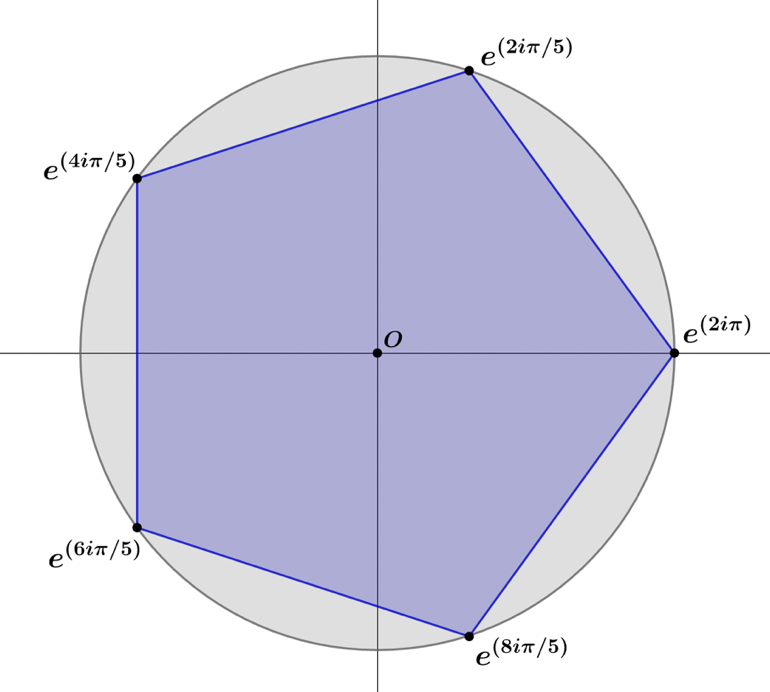
Figure 1.7.18 – The inscribed regular pentagon in the complex unit circle, representing the geometric prime.
has the distinct set of eigenvalues , representing the complex number . As expected, since this is a geometric prime, all generators have the same set of eigenvalues, where the set of Lie algebra generators is
(1.7.204)
The inscribed regular pentagon representing the geometric prime is presented in Figure 1.7.18, with each vertex valued at an eigenvalue from the set
(1.7.205)
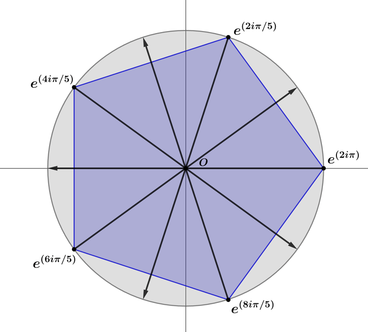
There are five ways to split the regular pentagon into two equal-sized portions, all of which involve extending a segment from each vertex to the midpoint of the opposing edge, known as the apothem. If this segment extends through the edge and to the boundary of the complex unit circle, it will intersect the boundary at the vertex's antipodal point, as seen in Figure 1.7.19.
Figure 1.7.19 – The symmetry of , seen as vectors that originate at each vertex,, extending past the midpoint of the opposite edge of the regular pentagon, and intersecting the boundary of the unit circle at the antipodal point,
We extend the group to its higher-dimensional generators by calculating the products of the anti-identity with the set of Lie algebra generators , which yields the set
(1.7.206)
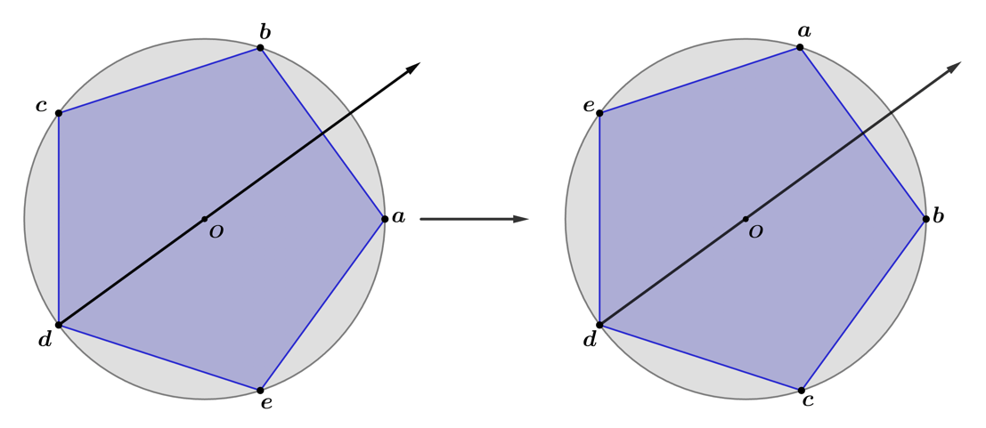
Each generator in the set acts to rotate four of the five vertices about an axis of symmetry of the regular pentagon seen in the previous figure. We take the second Lie algebra in the set above to consider the matrix-vector product
(1.7.207)
The result leaves the -vertex as unchanged, while the vertices and exchange, as do and . To best visualize the rotation, we represent the transform in the figure below, where the vertices reflect across the axis of rotation extending from .
Figure 1.7.20 – The rotation, with an axis of rotation along the -axis.
The set of Lie algebra generators act in a manner similar to the -type generators, where they have an axis of rotation and symmetrically rotate in the non-axis planes.
This unique symmetry of the regular pentagon contrasts with the two symmetries of the regular square, which were the even halving of the square from vertex-to-vertex splitting and mid-edge to opposing mid-edge splitting. This process can be continually repeated, by first creating the set of cyclic Lie algebra generators , then rotating each element in the set by the anti-identity to build all the higher-order groups.
We return to consider the characteristic polynomials of the primary Lie algebra generators of the set by finding the determinant of the matrix
(1.7.208)
for the result , representing the characteristic polynomial. Given that the set represents a geometric prime, we know that all characteristic polynomials will be the same except for the identity element, whose characteristic polynomial is
(1.7.209)
with a set of eigenvalues that are all equal to one, To make it clear to the reader, solutions to the characteristic polynomial set equal to zero are the eigenvalues of the matrix. This also represents a polynomial expression with variables that can take on matrix values. For instance, the characteristic polynomial can be expressed as
(1.7.210)
where represents a matrix variable, and is the square identity matrix. All the Lie algebra generators from the set are solutions to this matrix polynomial above, which we can demonstrate with the generator by setting , and calculating as follows
(1.7.211)
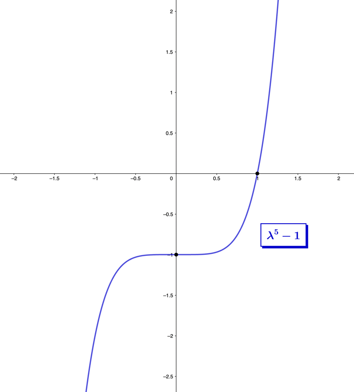
For the above, is equal to , given that each successive power shifts the entries to the right by one off-diagonal, which after five shifts returns to the identity generator. In Figure 1.7.21, we plot the characteristic polynomial in the real domain, where the function has a root at . We recall that the other solutions in the complex plane are the remaining eigenvalues from the set
(1.7.212)
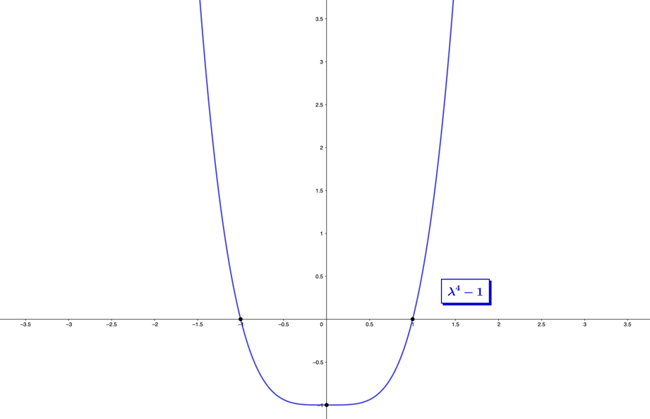
The plot of the characteristic polynomial function , like the function , is anti-symmetric about the vertical axis, given that it is an odd-powered polynomial. We compare this to the even-powered characteristic polynomial of the Lie algebra, whose result was found to be
(1.7.213)
Figure 1.7.21 – Plot of the characteristic polynomial function in the real domain with its real root equal to the real eigenvalue from the set .
The characteristic polynomial function represents an even degree polynomial, and in Figure 1.7.22, we can see the function's plot has symmetry about the vertical axis, and in the real domain, the function has two roots at .
Given that is a composite number, we find that there are, in addition to the identity's characteristic polynomial two others: the first generated by the positive and negative minimal elements,equaling the result , and the second is based on prime composition , where . We find by calculating the following determinant
(1.7.214)
a characteristic polynomial equal to , where the portion in parenthesis is equal to the characteristic polynomial of the primary generator, belonging to the geometric prime set .
Figure 1.7.22 – Plot of the characteristic polynomial function .
Like the prime number composition , represents a prime characteristic polynomial composition, which we can express as follows
(1.7.215)
where denotes the non-identity unique characteristic polynomial of the geometric prime. We also use the following notation to express powers of
(1.7.216)
which will prove helpful as we look at more non-prime composite geometric numbers. A look at the set of generators representing the hexagon, , is seen below
(1.7.217)
and there are a total of four different characteristic polynomials in this set, which are the following
(1.7.218)
(1.7.219)
(1.7.220)
(1.7.221)
Of the four characteristic polynomials, two represent prime characteristic polynomial compositions as follows
(1.7.222)
where we can generalize the notation to
(1.7.223)
which holds for all prime characteristic polynomial compositions.
To represent the sum of all characteristic polynomials in the group, we create a group characteristic polynomial for the set , defined as
(1.7.224)
where the coefficients are determined by the number of times each characteristic polynomial appears in the set. In expanded form, the group characteristic polynomial is
(1.7.225)
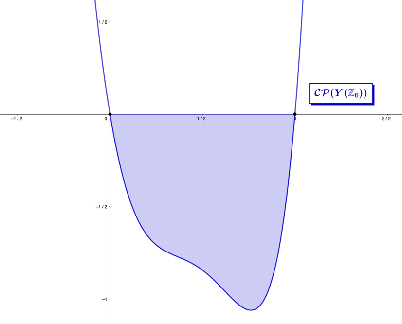
and plotted in the figure below, where the blue-shaded region represents where the function dips below the horizontal axis for values between and .
Figure 1.7.23 – Plot of the group characteristic polynomial function.
The area of this blue-shaded region is found by calculating the integral ,
(1.7.226)
whose result we see is greater than Below we list several integrals of the group characteristic polynomials with boundaries between and , up to the group , where prime numerator results are in depicted in bold:
(1.7.227)
(1.7.228)
(1.7.229)
(1.7.230)
(1.7.231)
(1.7.232)
(1.7.233)
(1.7.234)
(1.7.235)
(1.7.236)
(1.7.237)
(1.7.238)
(1.7.239)
(1.7.240)
(1.7.241)
(1.7.242)
At the onset, we find a high frequency of prime numbers for the numerators in the results, but after the integral this tendency appears to decrease. The non-prime integral results are a mix of rationals with even/odd and odd/odd values, while all the integral results of geometric primes have results that are odd/even rational number values.
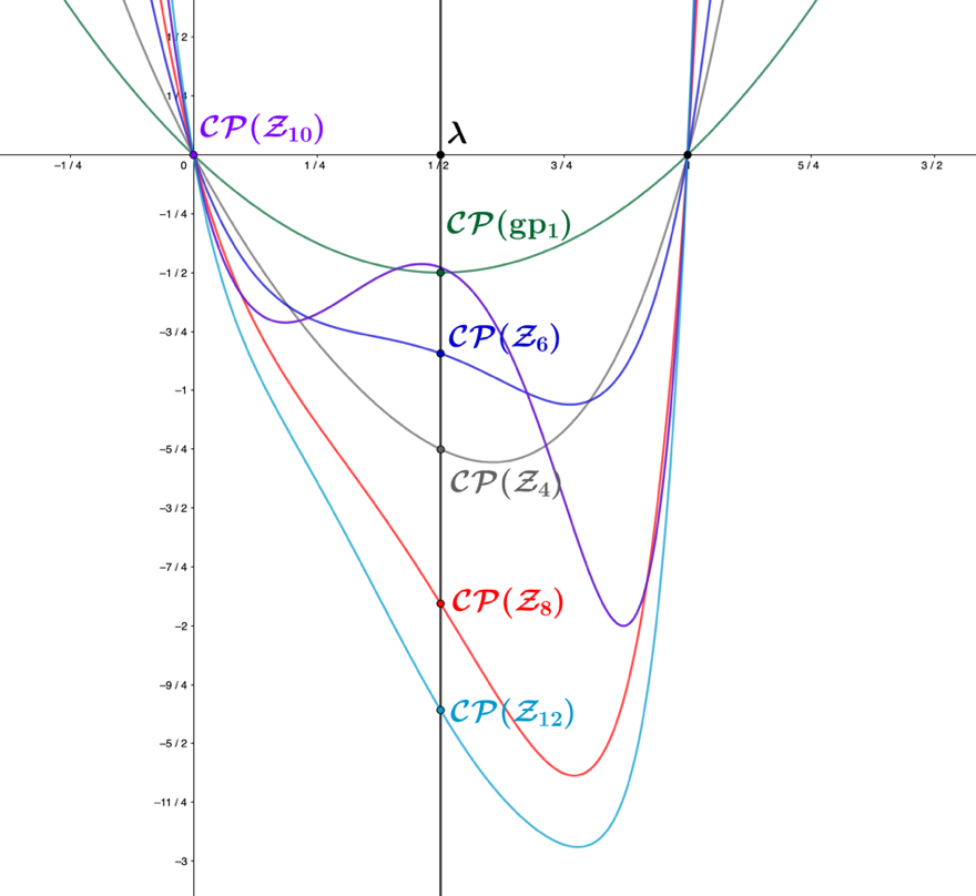
We plot in the following figure, the group characteristic polynomials for the first six even-numbered integers, seeing that each function has a global minimum on the interval and the global minimum of the geometric prime function is located precisely at
Figure 1.7.24 – Plots of the group characteristic polynomial functions for .
The group characteristic polynomials of the geometric primes have the following generalized form
(1.7.243)
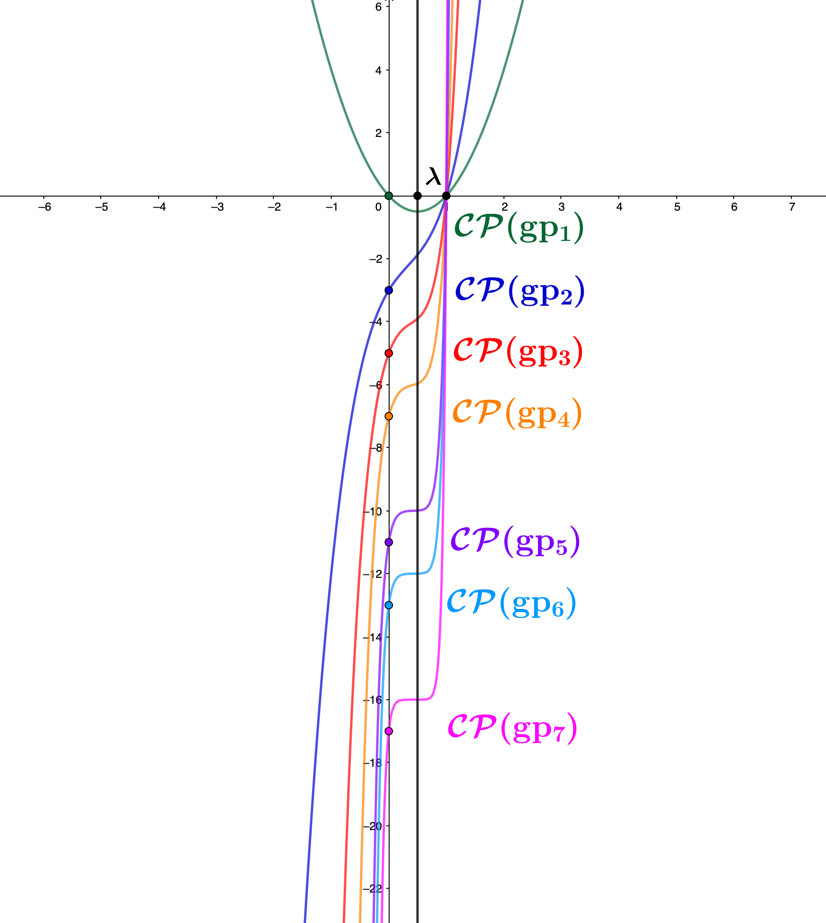
which is distinct as a polynomial and potentially a means to distinguish a prime number from a composite number by the graph of its function. Plotting the first seven geometric prime numbers below, the rapid flattening of the curves for each function centers around values of coinciding with vertical axis values at approximately the even integer preceding each , or around
Figure 1.7.25 – Characteristic polynomial functions for the set of geometric primes, ,.
We evaluate how closely the value at comes to each even number by solving the function , for
(1.7.244)
which for all primes except for , becomes
(1.7.245)
where the negative-valued integer term, appears in the result, and the term reduces in size exponentially by . Using the example for the fifth geometric prime , where , we find the result
(1.7.246)
which we can see is very close to the value , for In the figure, it is also apparent that the odd-valued functions cross the vertical axis at their negative integer values, and mathematically, we can understand why this is the case by solving the following expression
(1.7.247)
for the trivial value
(1.7.248)
and given is odd for all , we have that , and we find
(1.7.249)
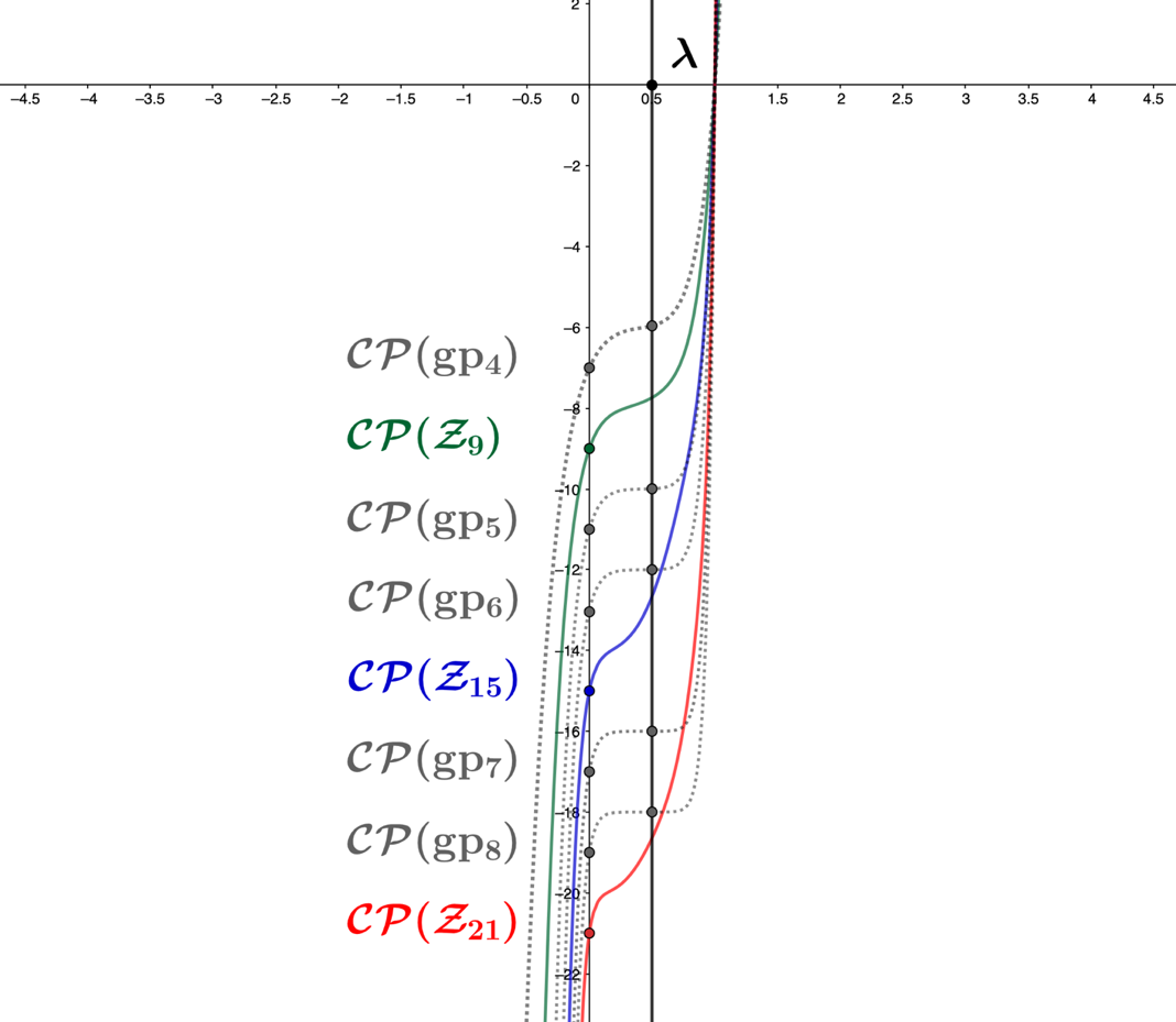
Figure 1.7.26 – Plots of the group characteristic polynomial functions for the set of odd-valued non-prime functions and the neighboring set of prime-valued functions .
To show how the functions differ from the odd non-prime composite functions in the interval , we plot in Figure 1.7.26 the set of functions for, and compare this to the set , for . We mark the point where the geometric prime characteristic polynomial functions cross the strip at . All of the functions intersect the vertical axis at the negative value of their natural number at . As mentioned previously, at the point of the plot when , the functions are all close to the intersection point with the integer value . The non-prime group polynomial functions cross the adjacent integer threshold for , on the interval
There is a geometric basis to our definition of the group characteristic polynomials related to the primary generators. For composite numbered groups, lower-ordered polygons will exist that evenly divide the -gon defined by its group, while the prime number groups consist solely of their unique primary generators, , along with the identity generator . The number of primary generators for lower-ordered polygons inscribing the group's -gon represent the constants in that group's characteristic polynomial. This is in addition to the unique primary generators of the -gon itself, calculated as
(1.7.250)
where denotes the number of primary generators of the -gon and are lower-ordered primary generators that inscribe the -gon geometry. An example helps to visualize what this means we look at the group, for which, the dodecagon is its defined -gon, and its group characteristic polynomial is
(1.7.251)
where we have arranged the polynomial by order of the 's. Each term in the polynomial represents the primary generators of the sub-ordered polygons that inscribe the dodecagon. The integer can be divided without remainders as follows:
(1.7.252)
Each division represents the polygon defined by this number of vertices and the number dividing will represent the exponent of each primary generator equation. Each primary generator equation will have the form
(1.7.253)
where the exponent represents the number of primary generator vertices for the inscribed polygon representation, is the number of primary generators in the polygon, and the exponent represents the number of times this lower-ordered polygon divides the higher-order -gon. For , all the primary generator polygon terms are presented below that evenly divide the geometry of ,
(1.7.254)
where the leading constants for each term define the primary generators that the polygon has. Each primary generator, by way of successive powers, can generate all the elements in its subset, and to ensure clarity for the reader, we present the primary generators for each lower-order polygon above:
(1.7.255)
To determine the value of the constant, we solve our sum
(1.7.256)
and geometrically, the result represents the four vertices of the dodecagon that are not vertex points of identity-aligned sub-polygons, which as a set are the point, the line, the equilateral triangle, the square, and the regular hexagon. With the constants determined, we can now express the characteristic polynomial as
(1.7.257)
which is presented in the figure below in the inscribed geometry representation.
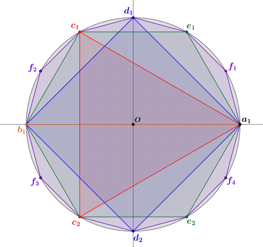
Figure 1.7.27 – The inscribed geometry of . Colored diamonds on the boundary represent the primary generators of the lower-ordered -gons, and purple circles represent the primary generators of the -gon.
Group characteristic polynomials are comprised of terms stemming from the sub-geometries that inscribe their geometry, weighted based on the number of primary generators in the set of elements from those sub-geometries. As we are aware, a geometric prime will have a total of primary generators, and in the previous example, the terms were and respectively. When higher-ordered geometric primes are present in a group's characteristic polynomial, these tend to be weighted more heavily than a composite Geometric Number for degrees of and that are in proximity.
To finish the section, we look at the group characteristic polynomials' terms, which represent the embedded minimal elements of the sub-geometries that comprise that group's order. As stated before, the terms in a group characteristic polynomial will have the form
(1.7.258)
and the unique minimal element to the embedded degree geometry is
(1.7.259)
representing either the first vertex of the -gon that is positively oriented from the identity, , or the first vertex which is negatively oriented from the identity, The minimal elements and the other primary generators are solutions to the characteristic polynomial equation . The minimal elements yield a solution to this equation, having a winding number of one around the complex unit circle for the evaluation of the characteristic polynomial equation
(1.7.260)
For primary generators, that lie on the upper half of the unit circle for positively oriented solutions, or the lower half for negatively oriented solutions, the winding numbers will be equal to the value
(1.7.261)
for which, the result represents a distance factor the primary generator is from the minimal element
(1.7.262)
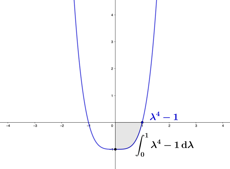
Figure 1.7.28 – Plot of the characteristic polynomial , in blue, and its integral , the area in black.
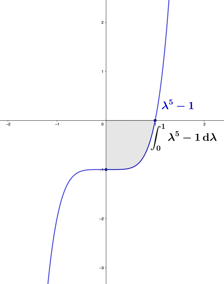
Figure 1.7.29 – Plot of the characteristic polynomial , in blue, and its integral , the area in black.
In *Figures 1.7.28 & **1.7.***29, we consider the graphs of the characteristic polynomial equations ,, where the blue areas represent definite integrals of these equations from to , with the following results
(1.7.263)
(1.7.264)
The areas bound by the characteristic polynomials between and can be generalized to the form
(1.7.265)
and if we consider the negative-valued characteristic polynomial,
(1.7.266)
this equals one-half the value of the inverse triangular numbers found in the previous section
(1.7.267)
With the Euler product in mind, we can express the harmonic series in terms of the characteristic polynomials of the geometric primes
(1.7.268)
or as the product
(1.7.269)
The term in the geometric prime group characteristic polynomial
(1.7.270)
is the same as the term in Wilson's theorem, showing the connection between the geometry of the minimal element and the more conventional approach to introductory number theory. Details about number theory and Wilson's theorem are in the remaining sections that follow.