This section returns to some of the concepts covered in Section 1.7.2, involving aspects of the dimensional transformation mapping . This will help us better understand the nature of light and consider how the mathematical framework we have been working with is causal to the physical phenomenology perceived around us. We start by looking at the first cone number in the positive orientation from the identity, which has the following equivalence expression
(1.8.244)
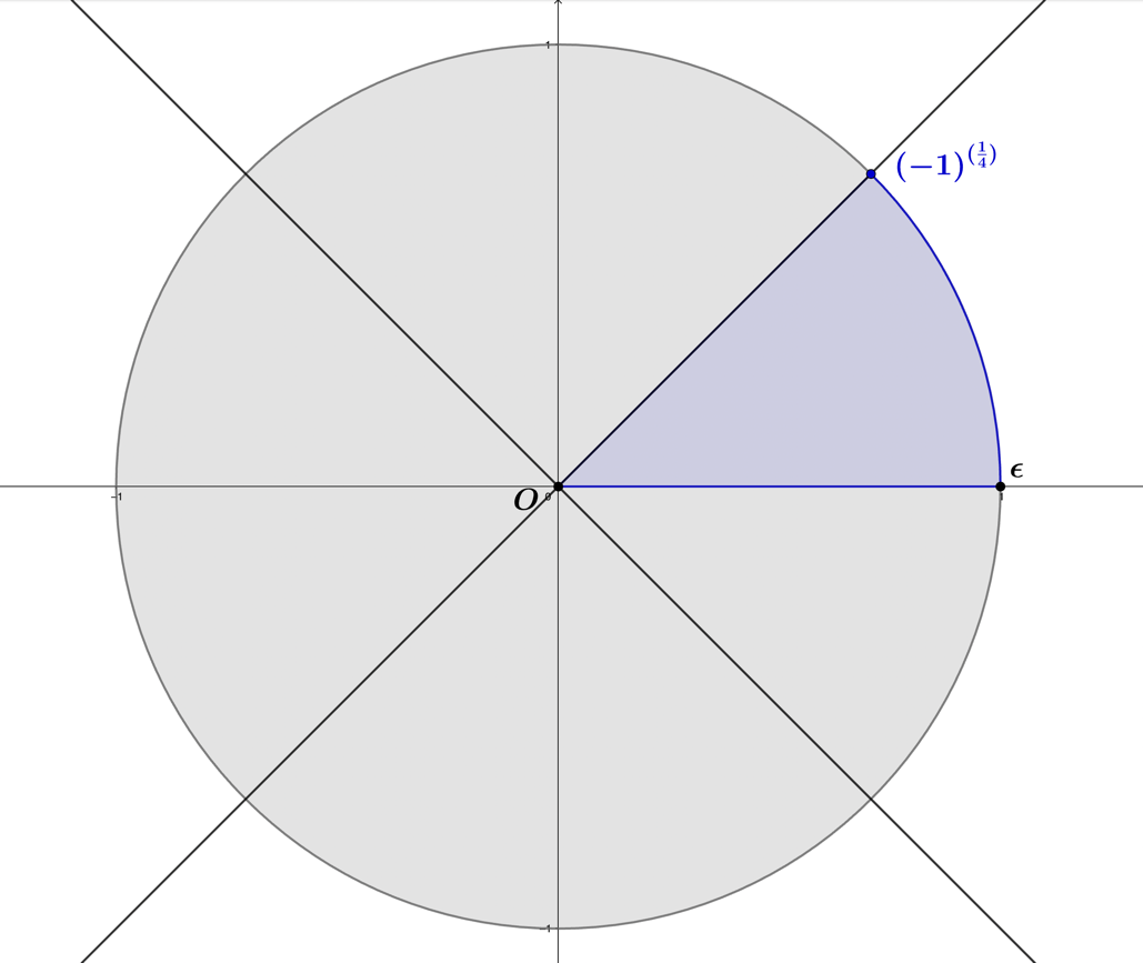
and point on the complex unit circle is depicted in Figure 1.8.10. Based on the two previous sections, this number should stand out as the positive minimal element of the inscribed octagon, which, in mathematical notation, is
(1.8.245)
and this cone number belongs to the set of Lie algebra generators
(1.8.246)
Figure 1.8.10 – The cone number on the complex unit circle.
Each element in the set above has an matrix Lie algebra generator representation, which can be seen using the example for the algebra
(1.8.247)
where the set of elements can be generated by , given that by default, the positive and negative-valued minimal elements are primary generators, The matrix has eigenvalues representing vertex positions in the complex unit circle, comprising the set
(1.8.248)
The primary generator element subset represents the cone numbers
(1.8.249)
and the remaining elements of are the axis numbers, which define the inscribed square geometric integer ,
(1.8.250)
The matrix representation of the primary generator has a total of entries, which can take on values of either or , signifying bits of information. As a primary generator, the spatial arrangement of the non-zero entries also encodes the entire group by way of the multiplication operation . As a group, is encoded in bits of information, which can be seen when we consider the eight cyclic shifts of the Lie algebra generators in binary
(1.8.251)
and given that there are eight non-zero elements in each cyclic shift matrix, there are bits of information.
Previously in the chapter, we considered dimensional transforms of numbers, recalling the following example for the dimensional mapping from a complex number to a real matrix
(1.8.252)
We apply the same dimensional transform mapping in the opposite direction for our minimal element , by using the mapping notation
(1.8.253)
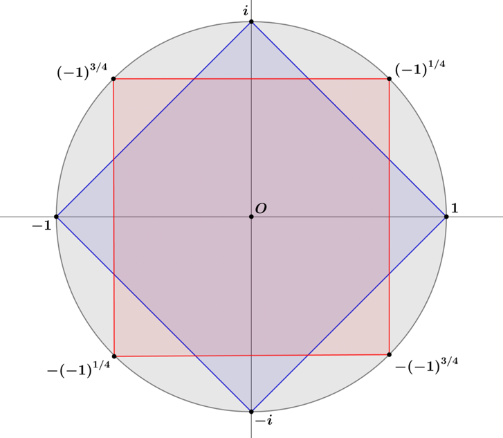
We have gone from an sized matrix to a matrix and introduced a negative-valued integer in the position of the mapped result. As we know, the matrix represents the inscribed square, and a look at the eigenvalues of the matrix, reveals the cone numbers
(1.8.254)
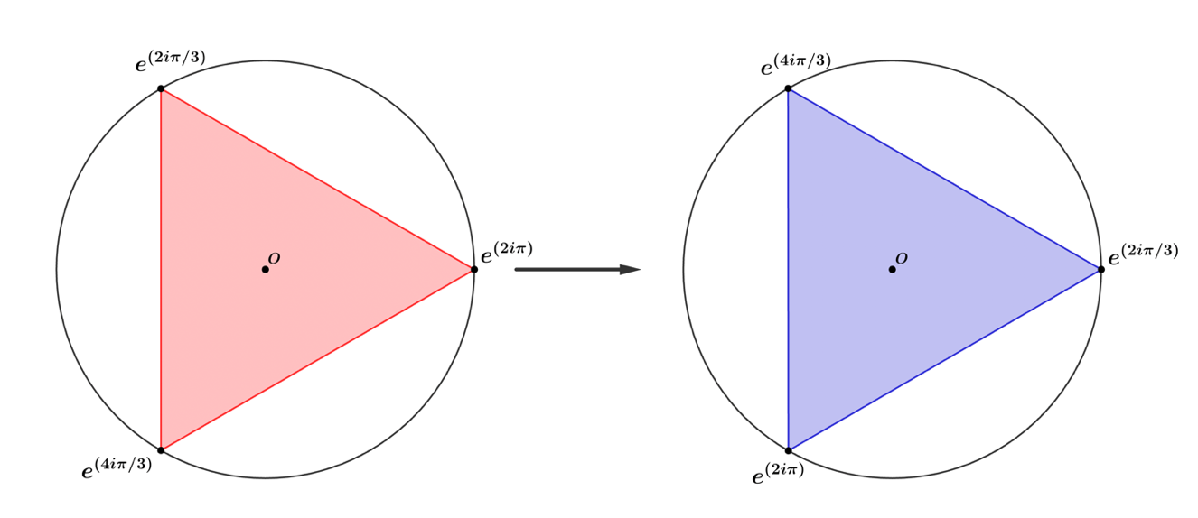
The eigenvalues signify that the inscribed square has been rotated by radians when compared to , where is seen in the following figure as the red square, and as the blue square.
Figure 1.8.11 –The inscribed position of in blue, is rotated to the position in red.
The generator forms the octagon by way of its successive powers, which generates the following set of eight unique elements
(1.8.255)
In the set above the eigenvalues of the , elements are
(1.8.256)
which, together with the eigenvalues of the primary generator
(1.8.257)
encompass the eigenvalue set.
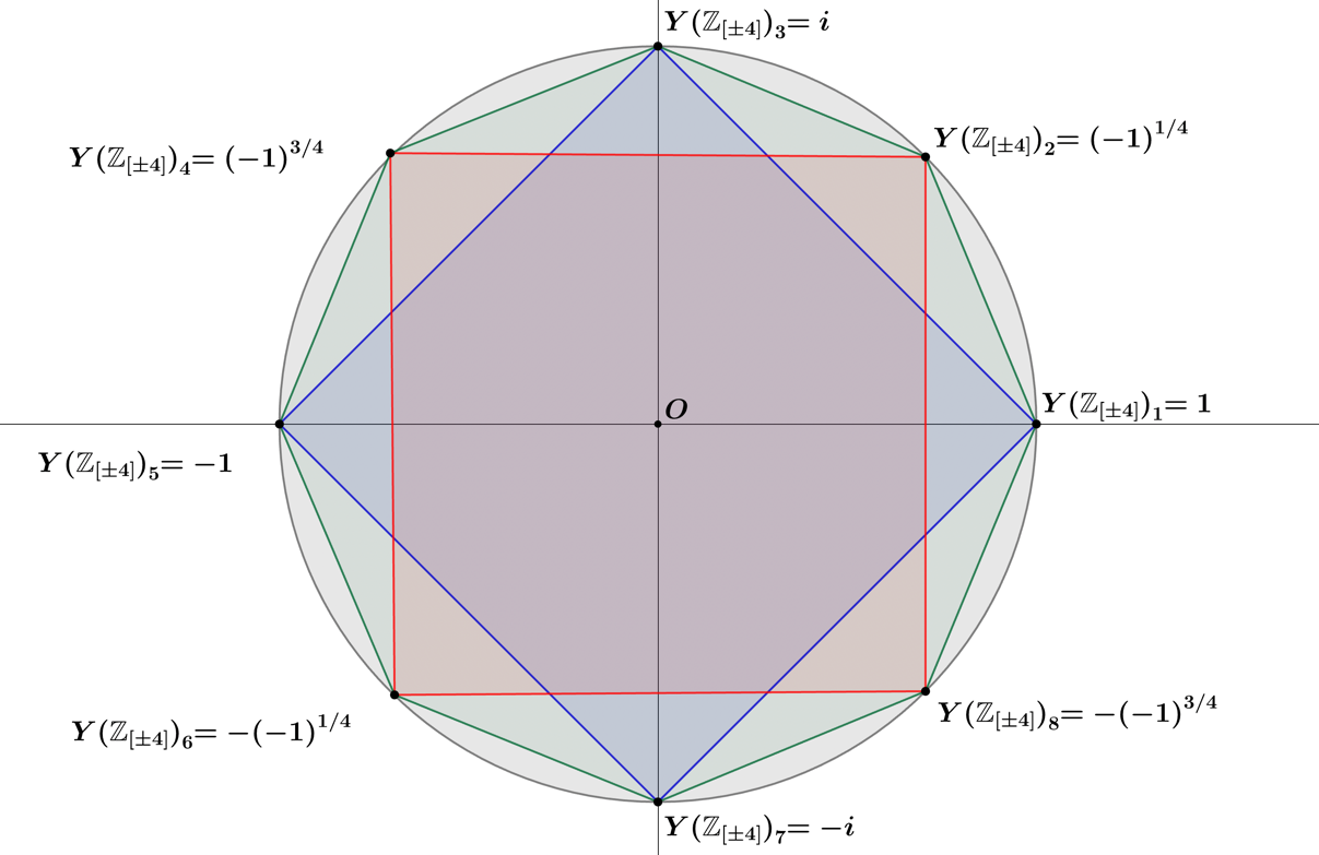
Figure 1.8.12 –The vertex values associated with the set of elements.
We show the inscribed geometry of the regular octagon, the result of the primary generator's rotations and represent the elements in the set. It may be counterintuitive at first, but if we first consider the and elements
(1.8.258)
to represent the vertex locations at and on the complex unit circle, the consistency as vertex locations is appreciated by squaring each
(1.8.259)
So, is found to equal the negative identity, which is the expected result given that and then we find , representing The set cycles twice in terms of shifts before returning to the identity element. The eight Lie algebra generators of the set can also be represented as the following binary set
(1.8.260)
where the directional arrow for signifies the above is a shifting set. Given that non-zero entries take on two values, , there are eight bits of information in each Lie algebra generator , which, when multiplied by the number of elements in , we find bits of information are present in the group, revealing that a conservation of information exists in the mapping As expected, in the set there are also four primary generators
(1.8.261)
which differ from the non-generators based on their lack of symmetry for non-zero entries about the diagonal and the odd number distribution of positive to negative values. These primary generators represent cone numbers given that when squared, all the resulting elements are imaginary-valued Lie algebras
(1.8.262)
evidenced by the fact that when squared, the elements equal the negative identity
(1.8.263)
The geometric integer set is contained in the set, , where is the subset
(1.8.264)
Geometrically is a subset since the vertices of the inscribed square, , are aligned on the four axes points of the complex unit circle and are limited to vertex rotations of radians, therefore, can be rotated in four different ways to align its vertices with the inscribed octagon. Next, we reduce the size of the dimension while conserving its information content with the mapping
(1.8.265)
where it is easy to verify that matrix represents a cone number by its square
(1.8.266)
and more specifically, that
(1.8.267)
since the positive rotation The set of Lie algebra generators is the following
(1.8.268)
which, like our other sets, contains a total of eight elements representing the octagon. The primary generators have the following cone number values for their eigenvalues
(1.8.269)
(1.8.270)
while the remaining elements have eigenvalues that are equal to the axis values of the inscribed square
(1.8.271)
where these axis numbers have only one unique eigenvalue. This lack of uniqueness of eigenvalues is a mathematical indicator that these are not primary generators of the set. As the reader may have guessed, we can also further reduce the dimensions of the matrix representation for the set to the form of the set . This represents the complete transformational mapping of the geometric integer to the complex plane and the set is comprised of the following Lie algebra generators
(1.8.272)
for which, each element in the set is a point on the complex unit circle, representing the eigenvalues of the geometric integer. The matrix representation of the minimal element we began with, is a complex number, and the dimension-reducing transform
(1.8.273)
makes this mathematically clear.
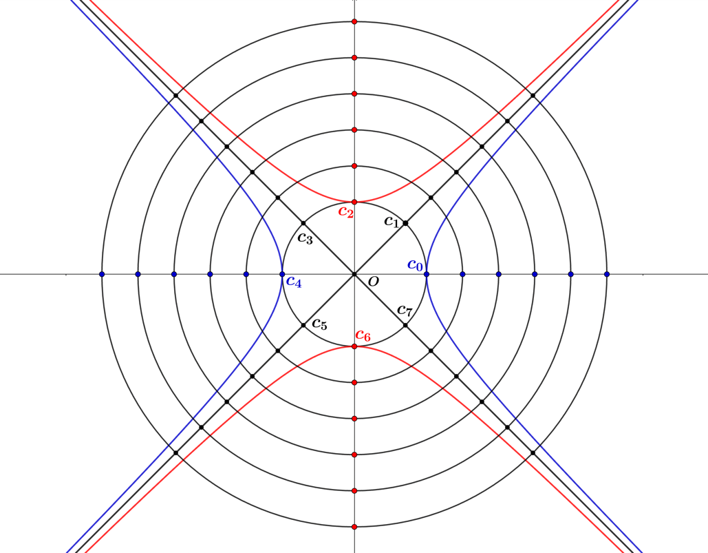
Previously mentioned was that the minimal element is physically associated with light. Expanding on this connection is appropriate with our background from the previous section on the geometric integers and primes. In physics, light, specifically electro-magnetism, is represented in the form of the group, which is consistent with the result we arrived at using our dimensional transform We have seen that there is a fundamental geometry that is central to the characteristics of groups, and the case for is no exception. Light is based on the first prime number , and the inscribed geometry of the geometric prime. Early in the book, we offered a similar representation to Figure 1.8.13 below, where the geometric forms of the complex circle, the hyperbola, and the hyperbola's asymptotes are presented. In the figure, we have labeled points on the unit circle using the notation , representing the ordered set
(1.8.274)
which can be seen to include points on the asymptotes and the axes. Also present in the figure is curvature, in the form of positive curvature for the unit circle, negative curvature for the hyperbola, and light having flat curvature as the perfect balance between the other two.
Figure 1.8.13 –Points in the complex plane from the light set radially projecting from the origin.
In 1905, Albert Einstein published a paper named "On the Electrodynamics of Moving Bodies"1, in which he proposed his theory of special relativity. The theory is based on the postulates that the laws of physics are invariant, and the speed of light is invariant for all observers. The impetus behind the theory stemmed from the compatibility issues that Newtonian mechanics had with Maxwell's equations, and the theory corrects mechanics for bodies moving at close to the speed of light, often referred to as relativistic velocities.
Special relativity is a consequence of hyperbolic geometry. We will touch upon the subject briefly and will ultimately go more in-depth into the subject matter in the ensuing books on physics in the Arithmoí series. The most common form of the Lorentz transformation representing velocity unique to the -direction is
(1.8.275)
where and , represent the two coordinate frames of an observed event, for the stationary frame , the moving frame , the speed of light , and the Lorentz factor
(1.8.276)
Space and time are one and the same, and by choosing to measure them with the same units, , we replace the time variable in the Lorentz transformation to measure the coordinate frames of our observed result as and , where the transformations become 2
(1.8.277)
The symmetry between the spacetime and velocity transforms becomes more evident in the expressions above. There are also inverse Lorentz transformations, given that no privileged reference frame exists in the special relativity theory. These inverse transformations are found simply by solving the transformations above for and
(1.8.278)
and these represent the frame moving with a negative velocity that is equal in magnitude relative to the frame. We substitute the term, , for, where is the rapidity term, and for the unit hyperbolic equation
(1.8.279)
we solve for as follows
(1.8.280)
for which is the hyperbolic Lorentz factor, , and we set the equivalence
(1.8.281)
The following equivalence is then the case for the function
(1.8.282)
and now, we can substitute our hyperbolic equivalents back into the transformations
(1.8.283)
(1.8.284)
then put the hyperbolic transformations into matrix form, giving us
(1.8.285)
We take the example for a rapidity value of for , then being approximately equal to
(1.8.286)
and given that represents a frame that is moving at the speed of light relative to the observer's frame. We insert the value into the matrix form, to find
(1.8.287)
which signifies the values of the spacetime coordinates, distance, and elapsed time that the moving observer would record compared to the stationary observer. The inverse transformation can be found by left multiplying by the inverse of the transformation matrix
(1.8.288)
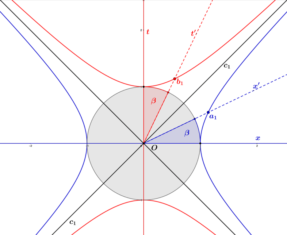
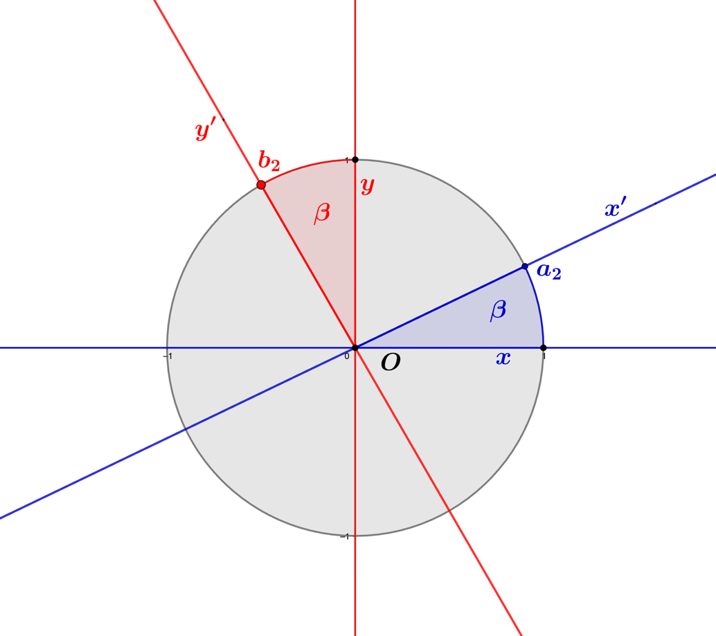
Figures 1.8.14,15 are plots of hyperbolic and Euclidean rotations, which are both orthogonal rotations in their respective geometries. In the hyperbolic case, two lines are orthogonal when they are reflections across the asymptote of the specific hyperbola. The asymptote found in Figure 1.8.14 is labeled , and represents the cone number as the speed of light. Hyperbolic orthogonality is central to special relativity for defining simultaneous events, where two events will be simultaneous when orthogonal to a specific timeline.
Figure 1.8.14 –Preserved hyperbolic orthogonality for the rotation with
The hyperbolic rotation in Figure 1.8.14 represents the inverse transformation for values of and , which are of equal magnitude. By choosing , this implies that elapsed time and distance are equal to , and calculating its matrix-vector, we find
(1.8.289)
which signifies the spacetime coordinates for an event seen by an observer in the frame was seen for the same by the observer in frame for coordinates
Figure 1.8.15 –Preserved Euclidean orthogonality for the rotation with .
More evidence that hyperbolic geometry truly underlies special relativity is found by looking at the Lorentz factor
(1.8.290)
for which, values of are expected to be entered for If the value for the velocity is entered as equal to the speed of light, , the Lorentz factor is infinite
(1.8.291)
and for superluminal values where , the Lorentz factor becomes imaginary valued
(1.8.292)
The hyperbolic rotation in Figure 1.8.15 represents the inverse transformation for values of and , which are of equal magnitude. By choosing , this implies that elapsed time and distance are equal to , and calculating its matrix-vector, we find
(1.8.293)
which signifies the spacetime coordinates for an event seen by an observer in the frame was seen for the same by the observer in frame for coordinates Evidence that the hyperbolic geometry is truly what underlies special relativity is found by looking at the Lorentz factor
(1.8.294)
into which values of are expected to be entered for If the value for the velocity is entered as equal to the speed of light, , the Lorentz factor is infinite
(1.8.295)
and for superluminal values where , the Lorentz factor becomes imaginary valued
(1.8.296)
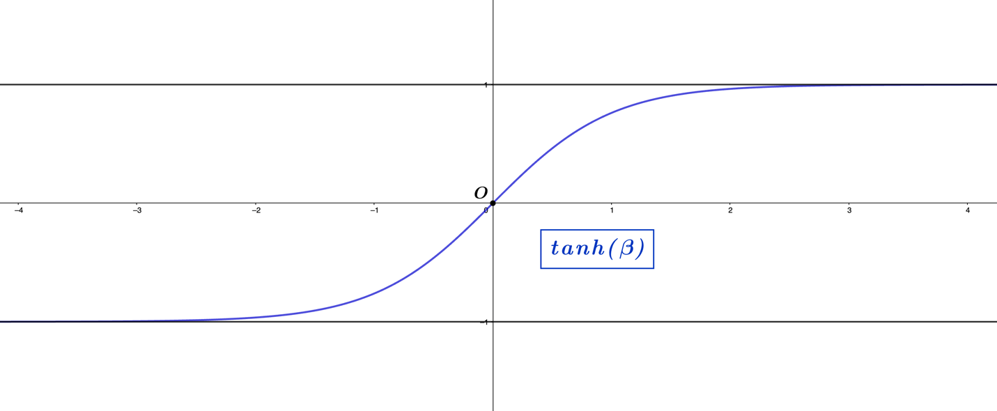
The function represents the ratio of the hyperbolic functions , and inherent in its mathematical form, it only approaches the value of one as
(1.8.297)
and negative one as
(1.8.298)
where these limits can be seen clearly in the graph of the function in the following figure.
Figure 1.8.16 –The plot of the function.
So, the hyperbolic form of the Lorentz factor
(1.8.299)
is not predicated upon entering a velocity less than the speed of light, and instead, we can see that is the result of hyperbolic geometry, and more precisely, it is the function. Geometrically, as the rapidity becomes larger, the degree of negative curvature decreases, and as , the curvature becomes flat, like that of the light asymptote.
Returning to the set of light elements
(1.8.300)
we consider the positively oriented minimal element where its successive powers can be seen to move along the axes and light asymptotes, seen by its ability to generate the set
(1.8.301)
This axis-asymptote propagation characteristic is how light moves mathematically and physically, which differs significantly from the phenomenology of massive objects bound by the relativity inherent to hyperbolic geometry. Light is outside of the geometric confines of spacetime, but, at the same time, it moves freely through the spacetime geometry.
Light is central to gaining a reasonable understanding of the universe, and any theory that does not consider its importance will be woefully incomplete. In Chapter 4, we consider conic sections, notably the light cone, which was significant because the light cone generated the subgroup. This subgroup stands out, given its distance metric is Euclidean, and in real space at non-relativistic velocities the world around us appears distinctly Euclidean. Light does not just represent a velocity limit for massive objects in space or photons/electromagnetic waves; it is mathematically responsible for creating the physical spaces in which we exist. This not only includes the real space we move around in, but also the imaginary space in which we move through time.
To understand the mathematics behind light, we return to the geometric integers to consider the dodecagon formed by cyclic rotations of the equilateral triangle. The geometric prime set had three unique elements, which coordinated with the three cyclic shifts of its vertices inscribed in the complex unit sphere
(1.8.302)
The inscribed dodecahedron is represented by rotating the equilateral triangle by radians, seen as the transformation in the image below.
Figure 1.8.17 – The rotation in the complex unit circle.
The first matrix representation of the rotated minimal element from the set, we denote as follows
(1.8.303)
which has one imaginary entry, and the other two are cone numbers situated radians away. By finding the eigenvalues of the matrix, we find consistency with the vertex positioning depicted in the figure above
(1.8.304)
which are all solutions to its characteristic polynomial
(1.8.305)
To see the intuition behind the result for the eigenvalues, each of these are solutions to the equation . The eigenvalues are calculated as follows
(1.8.306)
for which, taking the determinant of the matrix yields
(1.8.307)
and the eigenvalues are the said solutions to this characteristic polynomial in the complex plane. As we have seen previously, the matrix is also a solution to the characteristic polynomial, given that
(1.8.308)
We generate the subgroup by taking successive powers of the minimal element, to find the following set of twelve elements, where presents a positively oriented rotation,
(1.8.309)
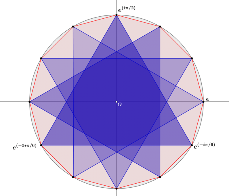
Geometrically, these are represented in the figure below, where each vertex may orient in one of twelve possible positions on the complex unit circle.
Figure 1.8.18 –The inscribed geometries of the set as
equilateral triangles inscribed in the dodecagon.
The group characteristic polynomial has remarkable symmetry, seen by the following
(1.8.310)
which represents the composition of the following subgroups of the geometric prime
(1.8.311)
(1.8.312)
(1.8.313)
(1.8.314)
The elements in the distinct subsets have determinants equal to in the expression . By its symmetry, the group characteristic polynomial reduces to the simplified form
(1.8.315)
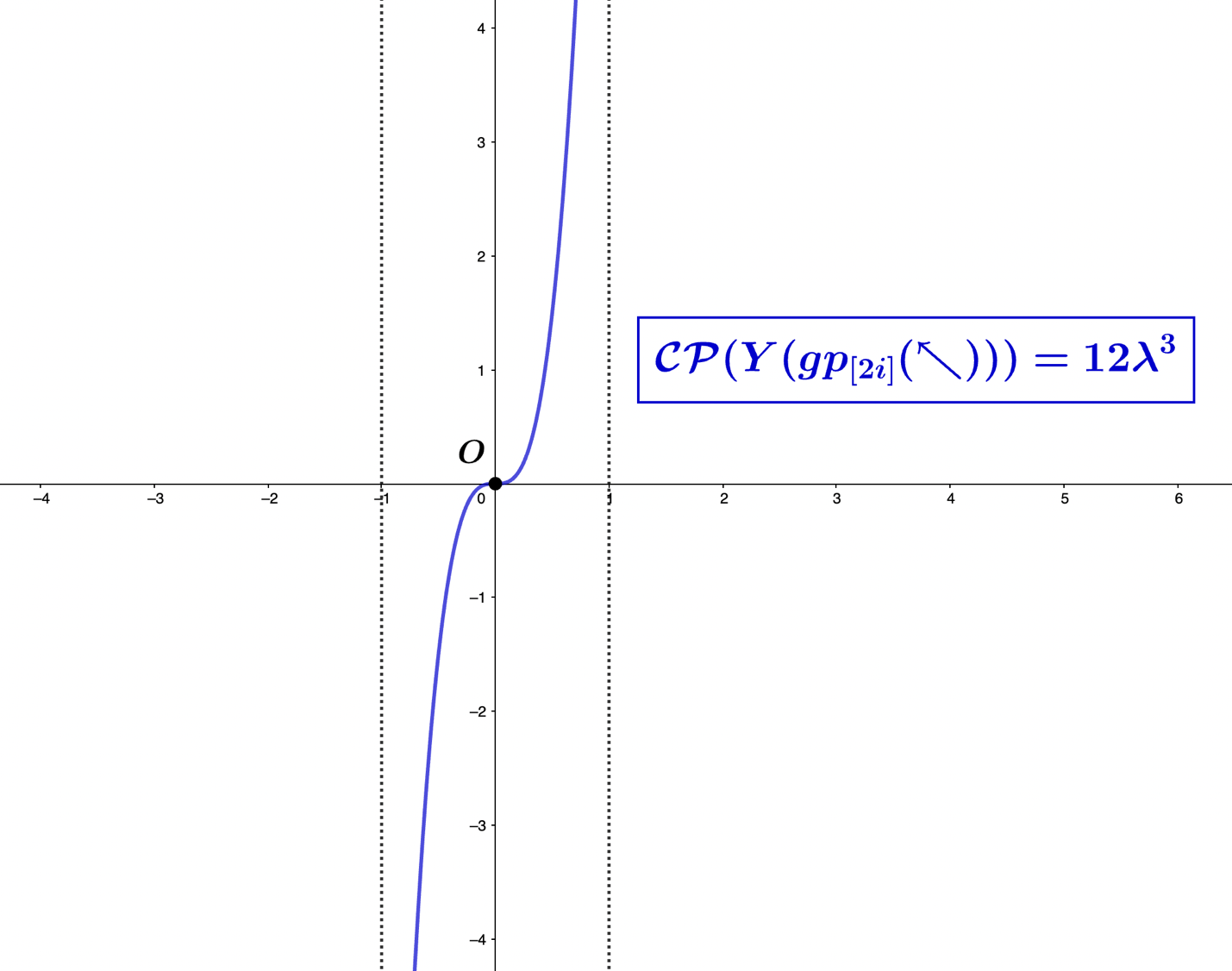
showing its dodecahedron characteristic form. Only the trivial solution exists for the characteristic polynomial equation signifying that the function crosses the real-axis only at the origin, as seen in the figure below.
Figure 1.8.19 –The plot of the group characteristic function
The net-zero characteristic is present in the graph above, meaning that for any point on the positive portion of the curve, there is another point on the negative portion that, when added to it, will equal zero. In other words, the characteristic polynomial is symmetric about the horizontal axis. Net-zero is essential for any theory of everything to be consistent mathematically and philosophically. Theories predicated upon a universe springing from the zero-point without a net-zero balance of its parts equates to the free-lunch model, for which any claim of causality is void. The cyclic group nature is inherent in the elements of the set, appreciated by first defining its subsets of elements
(1.8.316)
(1.8.317)
(1.8.318)
(1.8.319)
These can be situated into an array as
(1.8.320)
where the elements of each subgroup are arranged in three-element cyclic diagonals and the define the minimal elements, or, in other words, the primary generators. For clarity, we note as an example that Now, we take the subgroup elements found in the upper-left sub-matrix and define the minimal element subgroup, as
(1.8.321)
Successive powers of the minimal element subgroup will form a cohesive twelve element supergroup, composed of the following elements
(1.8.322)
This has a very similar structure to the set it was derived from, evidenced by the repeating three-element cyclic diagonals, the presence in the bottom half of the negative-valued elements coinciding with respective elements in the top half, and the presence of axes identities in the right-most column.
The supergroup process can be repeated indefinitely, considering the set can be arranged into the array
(1.8.323)
where the minimal element subgroup can also be defined as
(1.8.324)
whose successive powers also form the twelve element set
(1.8.325)
The minimal element is orientable in the other dimensions of , and our initial minimal element can be distinguished as
(1.8.326)
where presents a positively oriented rotation. The minimal element is the transpose of
(1.8.327)
has the same eigenvalues as
(1.8.328)
and the set of elements generating , is the following
(1.8.329)
The remaining complex dimension has the following minimal element
(1.8.330)
which has the following relationships with the other complex dimensional minimal elements
(1.8.331)
(1.8.332)
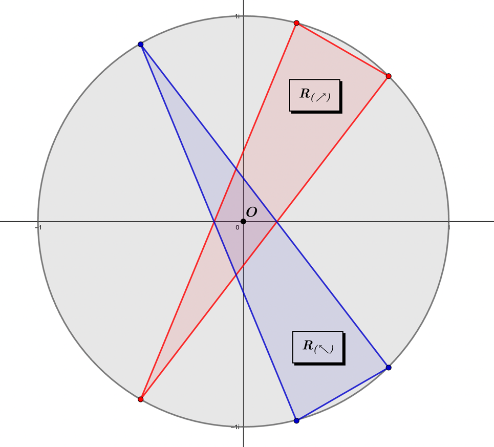
and the rotation matrices, represent oriented triangles in , given the eigenvalues for both are .
Figure 1.8.20 –The inscribed triangular rotations matrices and
Although may appear different from the other minimal elements, and , its eigenvalues are the same
(1.8.333)
which is the case given that a diagonalized matrix has its elements as eigenvalues. Graphically we can represent the two matrices, , which rotate and to , as points on the complex unit circle (Figure 1.8.20).
The set of elements generating , is the following
(1.8.334)
and the set of all sets , all have the same group characteristic polynomial
(1.8.335)
which, as we are aware, reduces to
(1.8.336)
The dimensional transform matrices are defined as
(1.8.337)
which, when mapping similar pointing arrows, rotate the minimal elements. The product of with matched matrices
(1.8.338)
will yield a set that includes all the cone generator Lie algebras, seen by presenting the composition of elements for each subset
(1.8.339)
(1.8.340)
(1.8.341)
In the subset, the square of the last element in each row is as follows:
(1.8.342)
where all are consistent with matrix representations of the complex numbers With the subset results after the dimensional transformation, a primary generator, that is alone capable of generating all the other elements, does not exist. Using the example of the transformed minimal element
(1.8.343)
the generated set from the result , has the subset representation
(1.8.344)
which contains the two cone portions oriented with positive and negative imaginary axes. Also present in the subset is the negative minimal element
(1.8.345)
which is bound to the same subset, given that its generated set is the same
(1.8.346)
Next, we take the transformation of the minimal element
(1.8.347)
which is equal to the cone portion oriented with the negative real-axis, and its generated set, contains only two elements, itself and the identity
(1.8.348)
We find the same holds for transforming the minimal element
(1.8.349)
which also has itself and the identity in its generated subset
(1.8.350)
So, a beautiful thing happens in the dimensional transformation process, where subspaces are formed with elements bound in the subspace.
The light numbers can take on many forms as matrix representations, and we use the example for the minimal element , having the matrix representation
(1.8.351)
which has eigenvalues equal to and its characteristic polynomial is , all of which are consistent with its nomenclature . Its generated set is composed of the following six elements
(1.8.352)
and we take the dimensional transformation of the set to find
(1.8.353)
The eigenvalues of four of the elements in the set above indicate that these are rotation matrices,
(1.8.354)
(1.8.355)
where each of these matrices generates
(1.8.356)
(1.8.357)
(1.8.358)
(1.8.359)
Except for the identity matrices, all of these generators act to rotate/reflect in the and -planes by and . We select the two non-diagonal matrices from these sets with their axis oriented along the real -plane,
(1.8.360)
which are inversely related to one another, given that
(1.8.361)
and the eigenvalues of the matrices are
(1.8.362)
The light cone we first encountered in the chapter on conic sections oriented along the real -axis, is the result of the product of these two matrices, with the real-axis oriented generator from the set
(1.8.363)
We rotate this cone section generator with the following matrix-matrix product
(1.8.364)
which results in the other light cone Lie algebra generator defined in the chapter on conic sections. We can now define the primary elements which form the light cone oriented in the -axis , as
(1.8.365)
which together form the following products
(1.8.366)
(1.8.367)
(1.8.368)
(1.8.369)
The Lie algebra results above are the versions of the generators seen previously in the book. Keeping the axis entry equal to the identity, we can represent this group of elements with variables , as
(1.8.370)
whose determinant represents the distance metric in the space
(1.8.371)
finding the Euclidean distance metric of the space we perceive phenomenally. With the resulting matrices formed by the light cone generator products, we define the set, as
(1.8.372)
The light cone along the negative real -axis is formed similarly, where we rotate the generators by
(1.8.373)
(1.8.374)
We define the primary elements which form the light cone oriented in the -axis , as
(1.8.375)
which together form the following products
(1.8.376)
(1.8.377)
(1.8.378)
(1.8.379)
We take these Lie algebra results to define the set as
(1.8.380)
which we find is equivalent to the set. It is important to note elements from the and the can generate other elements which depend on the order of the matrix product. For example, we consider the product of the following two elements
(1.8.381)
whose result has negative values in the bottom-right submatrix, compared with the positive element found
. These negative-valued elements represent rotations in the opposing directions, and by taking these into account, the light cone set is defined as the following set of Lie algebra generators
(1.8.382)
This is a beautiful mathematical result, given that the spaces created by two light cones, which are antipodal to one another, create seamless Euclidean space. So, moving in one space will feel like moving in the other space, and the two spaces will be indiscernible to anything bound in the subset. Light is responsible for this, particularly the cone numbers of light. The other light cones that are oriented in the -axes will yield similar sets, and we will dedicate a whole physics book on the subject in Arithmoí -Volume II, Part 1: "Phenomenology and the Geometry of Light".
To visualize the space along the -axis that the minimal elements
(1.8.383)
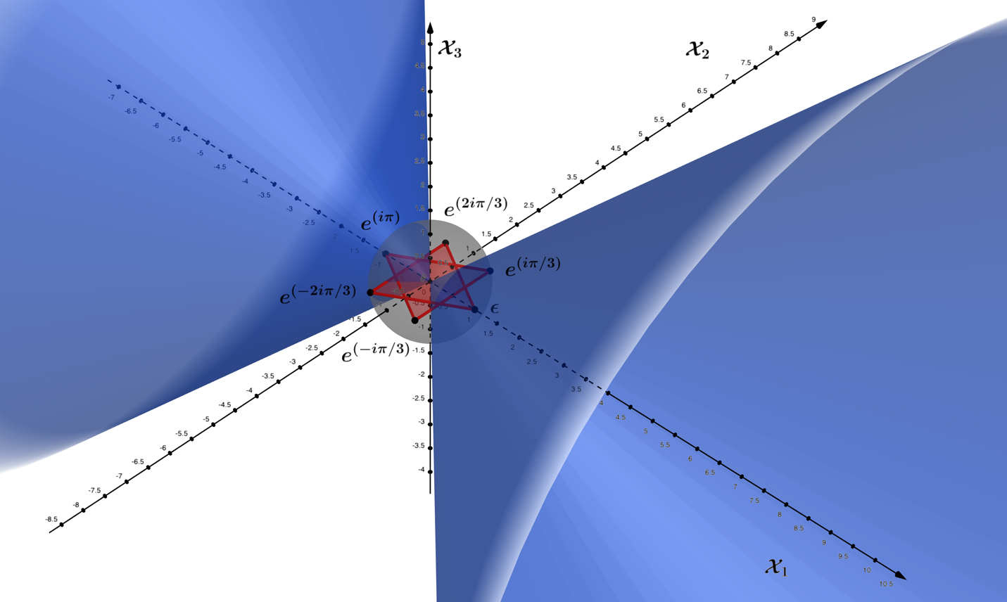
create, we plot in Figure 1.8.21 the eigenvalues of , as the vertices of the inscribed equilateral triangle. Emanating from the complex unit sphere in the positive and negative directions are the light cones of the -axis.
For completeness, we consider rotating to the and light cone sets, oriented along the and - axes, using the starting point of the light cone set
(1.8.384)
Figure 1.8.21 – Inscribed minimal elements and the -axis light cone. The positively oriented minimal element, , is pictured as the red triangle, and the negatively oriented minimal element, , is in blue.
Using the simple case of an -type Lie algebra
(1.8.385)
the and -types of Lie algebra will rotate as follows
(1.8.386)
(1.8.387)
where we see that rotates to the -type algebra, and rotates to the -type algebra. It should now be clear that the generators we have worked with throughout the book are the geometric prime in its simplest inscribed orientations, having eigenvalues equal to
We have seen before that changing the order of each product will yield rotations in opposing directions
(1.8.388)
(1.8.389)
Given these rotations, we know the right multiplication of the generator by some -type arrangement of elements will yield , and right multiplication by a -type arrangement will result in the generator.
The -type generator is found by taking the minimal element from the set, which has the matrix representation
(1.8.390)
then switch the values for the and entries, which gives us
(1.8.391)
As a primary generator, yields the following set
(1.8.392)
which interchanges , entries for the matrices in the left column (-type), and their transpose entries , in the matrices of the middle column (-type).
We define the following geometric prime rotation matrices using the notation
(1.8.393)
(1.8.394)
(1.8.395)
for which the values in the subscript indicate an oriented rotation from the -axis to the -axis. Each pairing of the rotation matrices are inversely related to one another, and these rotation matrices are derived from the products of the light cone segments as follows
(1.8.396)
(1.8.397)
(1.8.398)
The matrices represent -type geometric primes, which result from the products of the light cone segments. All these matrices have determinants equal to one, which is consistent with the value of light being set to unity. Given these matrices, we can define the following light cone segment rotations and respective inverse rotations as
(1.8.399)
(1.8.400)
(1.8.401)
The mathematical reasoning as to how the rotations work, is based upon the fact that each light cone segment will square to the identity, and the rotator is defined as . So, given that , the defined rotations will all generalize as follows
(1.8.402)
The straightforward matrix products
(1.8.403)
(1.8.404)
yield the positive and negative minimal elements. There are several ways to rotate the light cone sections, and we can choose to use the minimal elements, along with the rotators to define the following bijective rotation products
(1.8.405)
(1.8.406)
(1.8.407)
Note, as defined in the conic sections chapter, , have the same matrix representations
(1.8.408)
(1.8.409)
With light cone section rotations defined, we see that there is a very succinct interplay between the inscribed geometric primes and the light cone sections where the products of light cone sections yield inscribed geometric prime results, and these geometric primes also act to rotate the light cone sections themselves.
Up to this point, we have been considering light number solutions to the characteristic polynomial equal to axis numbers. We let the notation define the following -type matrices
(1.8.410)
for which all eigenvalue and eigenvector solutions will be as follows
(1.8.411)
(1.8.412)
(1.8.413)
The characteristic polynomials are found to be the following
(1.8.414)
(1.8.415)
(1.8.416)
which sum to the group characteristic polynomial
(1.8.417)
As stated earlier in the section, the numbers related to light will travel via asymptotes and axes. More specifically, the dimensionally transformed light numbers move in this manner. The inscribed geometry of the asymptotic light numbers will have Lie generators of the form
(1.8.418)
where the variables are the asymptote subset elements from the light set, which was defined earlier in the section, as
(1.8.419)
and the subset is
(1.8.420)
where the symbol denotes asymptotic and represents axes for the axis subset
(1.8.421)
which were pictured as the values in Figure 1.8.13.
We define the following minimal elements ,
(1.8.422)
which are both primary generators. We calculate the set the element, finding twenty-four elements in the set
(1.8.423)
The twenty-four elements are a due to the fact that the composite number is the result of the product of the prime numbers , and there is a symmetric distribution of the eight unique elements into subsets of the form
(1.8.424)
We consider the group characteristic polynomial
(1.8.425)
and given that for each subset, we have , the subset group characteristic polynomial is then equal to
(1.8.426)
Each value for is the result of rotation on the complex unit circle, and we can express each value as equaling
(1.8.427)
and the group characteristic polynomial can be found by the summation
(1.8.428)
We substitute , and calculate the sum to find the group characteristic polynomial reduces to
(1.8.429)
which is very similar to what we found for the group characteristic polynomial for our light cone numbers
(1.8.430)
This similarity is based upon the same symmetry in the elements of the group, and the two functions have the same plots except for a scaled difference of two. So, once again, we find the presence of the net-zero characteristic in the asymptotic light numbers.
The hyperbolic geometry of special relativity is also due to light numbers. Each hyperbola along the -axes is the dimensional transform of the set elements considered earlier
(1.8.431)
which also play an important role in light cone rotations. Using our rotation set notation, we can define the set as
(1.8.432)
given that this is a positively oriented rotation of the inscribed equilateral triangle. The dimensional transform will yield the -type Lie algebra generators
(1.8.433)
all of which are hyperbolic generators, seen by their variable-related matrix exponentials
(1.8.434)
So, the hyperbolic geometry that underscores special relativity is also a manifestation of light due to the geometric prime and its resulting dynamics. We also saw the role that these play in cone section rotations, and one way to think about this relationship is to consider the rotations matrices as a splitting of the geometric prime, which implies they are the result of light splitting. This notion can be expanded upon by considering that each matrix is the inverse of its pair, and the product
(1.8.435)
we see yields the identity of the set. The square for the segments is also equal to the identity
(1.8.436)
representing a symmetric splitting of the identity from the set, and this should remind the reader of the split complex number , whose square is equal to the identity as well. A closer look at the numbers using the example
(1.8.437)
has its axis represented by the entry, along with the submatrix in the bottom right corner, representing the symmetric identity split, manifested by rotating equal distances in radians away from in positive and negative directions. This submatrix is also another form of a split complex number, given that
(1.8.438)
which is consistent with our definition that , normally taking the matrix representation form
(1.8.439)
This representation obscures that it is also a symmetric splitting of the identity in positive and negative directions and rightfully sits in the space as
(1.8.440)
Further evidence that both split complex numbers are closely related is that they share the same determinants and eigenvalues
(1.8.441)
(1.8.442)
and subsequently have the same characteristic polynomial In the set, the non-identity elements should rightfully be seen as symmetric cyclic splittings of the identity, given that
(1.8.443)
and more precisely, both elements are positive and negative directional splits of the identity into thirds, which is the mathematical underpinnings for the fact that
(1.8.444)
The rotation matrices are closely related to the cyclic splitting of the identity above, given that each will also equate to the identity when cubed
(1.8.445)
and by associativity, all products will as well when ,
(1.8.446)
This applies to the products we encountered
(1.8.447)
where a three-way-splitting of the identity is causal to both
(1.8.448)
The logical conclusion is that all ontologically cohesive algebras are a split of the identity, known as the number one. This brings us full circle and back to the definition of the minimal element
(1.8.449)
which is exactly this splitting of the identity, given that , and the net-zero requirement for cohesiveness. For each , when , there exists its split analog, , for which the result of the following product always holds
(1.8.450)
How and why does the identity exist? The answer lies in the fact that it is the volume of the zero-dimensional point, which is indeed equal to , and is based on the volume definition of the -dimensional Euclidean ball
(1.8.451)
where is the radius, and is the gamma function. By solving for , we find the stated result
(1.8.452)
The net-zero splitting of the zero-dimensional point is causal to all the Lie algebras and groups we have considered in this book, and it is the origin of light in its raw and primordial form. The zero-dimensional point is eternal and uncaused, and with the birth and death of iterations of universes, it persists intact.
Light originates from inside of the singularity, where it is based on the dynamics of geometric primes and their polygonal forms, rotating in the complex unit sphere. Through the dimensional transformation, light manifests itself as spacetime, relativity, matter, forces, and all the other phenomena perceived locally. Inside the singularity, as the geometric prime gains more angles of freedom for its vertices, it takes on the composite geometry of the geometric integer and its polygon with that number of vertices.
This section considers the first and second geometric primes and their composite arrangements. The geometric prime will dimensionally transform to the prime and its composites, with an axis point that varies from fixed to geodesic on the complex unit sphere once exponentiated.
Albert Einstein (1905) "Zur Elektrodynamik bewegter Körper", Annalen der Physik 17: 891
Dray, Tevian, "The Geometry of Special Relativity", 2012, CRC Press