Masteries · Jason GlowneyArithmoí Book 1

Masteries

1.8.4 Relativistic Mechanics and the Unified Field

The form defin­ing the Uni­fied Field yields pow­er­ful physics right out of the gate. For in­stance, physics strug­gles to ex­plain the lo­ca­tion of the an­ti­mat­ter from the uni­verse's birth, where an­ti­mat­ter has the prop­er­ty of being op­po­site in charge to its matter part­ner. If an­ti­mat­ter and matter were to col­lide, they would mu­tu­al­ly an­ni­hi­late, pro­duc­ing in­tense energy in the process. Far-fetched ex­pla­na­tions have been pro­posed, e.g., it has been said that an asym­me­try ex­ist­ed at the moment of the uni­verse's birth, fa­vor­ing the num­bers of matter versus an­ti­mat­ter. These kinds of ex­pla­na­tions are a direct af­front to the net-zero prin­ci­ple, and, for this reason, they are in no way valid.

Ex­am­ples of matter/an­ti­mat­ter pairs are the elec­tron/positron (e,e)\ \left( e,\overline{e} \right), and the proton/an­tipro­ton (p,p)\left( p,\overline{p} \right), where we use the bar con­ven­tion over the par­ti­cle to denote an­ti­mat­ter. Math­e­mat­i­cal­ly, an­ti­mat­ter ro­tates in the op­po­site di­rec­tion on the in­fi­nite sphere of tan­gent spaces com­pris­ing the Uni­fied Field, which are the vacuum sin­gu­lar­i­ties at the Planck scale. Matter and an­ti­mat­ter share a mutual bound­ary on these in­fi­nite spheres of tan­gent spaces, but move around in op­po­site di­rec­tions, ac­count­ing for the dy­nam­ics of the vir­tu­al par­ti­cles of the vacuum. Ex­po­nen­ti­a­tion yields a radial ex­ten­sion away from the bound­ary of the sin­gu­lar­i­ty that can move inward or out­ward de­pend­ing on the mag­ni­tude of the real-valued com­po­nent. We present gen­er­al­ized math­e­mat­i­cal terms for form as 𝔣\mathfrak{f}, and 𝔣\overline{\mathfrak{f}} as its anti-form part­ner. In mm-di­men­sions, the Lie al­ge­bra for the form is de­fined as 𝔣(z)=𝔣(a+ib)\mathfrak{f}(z)= \mathfrak{f}(a + ib), and the anti-form as 𝔣(z)=𝔣(−a−ib)\overline{\mathfrak{f}(z)}= \mathfrak{f}( - a - ib), where a,b∈ℝ+m×ma,b \in \mathbb{R}^{+ m \times m}. Ex­po­nen­ti­a­tion of the Lie al­ge­bra of the form yields

exp⁡(𝔣(z))=ez=eaeib,\begin{array}{r} \exp{\left( \mathfrak{f}(z) \right) =}e^{z} = e^{a}e^{ib}, \end{array}
(1.8.71)

and for the anti-form

exp⁡(𝔣(z))=ez=e−ae−ib,\begin{array}{r} \exp{\left( \overline{\mathfrak{f}(z)} \right) =}e^{\overline{z}} = e^{- a}e^{- ib}, \end{array}
(1.8.72)

and for a≠0a \neq 0, the radial com­po­nent of exp⁡(𝔣(z))\exp\left( \overline{\mathfrak{f}(z)} \right) will be less than one, while the radial com­po­nent of exp⁡(𝔣(z))\exp\left( \mathfrak{f}(z) \right) will be greater than one. The pair rep­re­sents the sym­met­ric split­ting of the iden­ti­ty el­e­ment, and mutual an­ni­hi­la­tion occurs if the form/anti-form pair col­lides, given the result of their prod­uct

exp⁡(𝔣(z))×exp⁡(𝔣(z))=e0=ϵ.\begin{array}{r} \exp{\left( \mathfrak{f}(z) \right) \times \exp{\left( \overline{\mathfrak{f}(z)} \right) = e^{0} = \epsilon.}} \end{array}
(1.8.73)

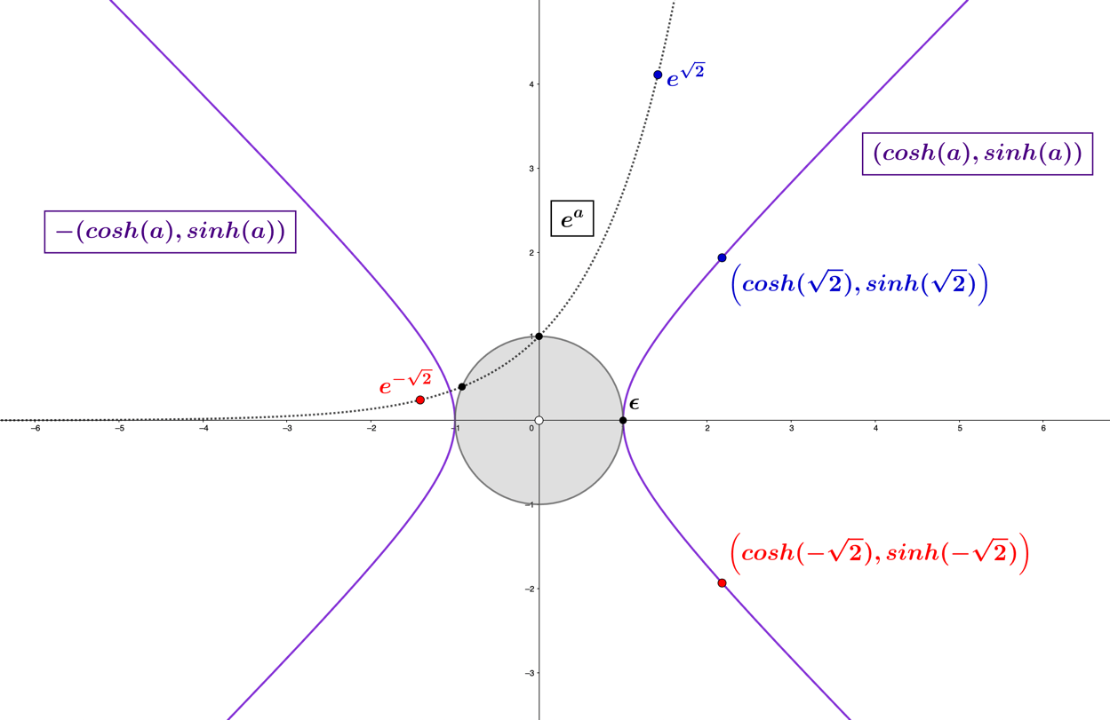
Math­e­mat­i­cal­ly, the answer to the ques­tion of an­ti­mat­ter's where­abouts is that it is present in the Uni­fied Field; only it exists at radial dis­tances of the Plank length and below. Im­por­tant to re­al­ize is that the dis­tance from zero to the Plank length holds just as much in­for­ma­tion as the dis­tance of the Plank length to in­fin­i­ty does. De­pict­ed in the fol­low­ing figure, we show a plot of the func­tion eae^{a} for a∈ℝa\in \mathbb{R}, which ad­heres to the net-zero prin­ci­ple given that it is a sym­met­ric split of the zero-di­men­sion­al iden­ti­ty, uni­tary in volume and lo­cat­ed at the func­tion's ver­ti­cal in­ter­cept.

The real ex­po­nen­tial por­tion e−ae^{- a} of the anti-form ex­pres­sion exp⁡(𝔣(z))=ez=e−ae−ib\exp{\left( \overline{\mathfrak{f}(z)} \right) =}e^{\overline{z}} = e^{- a}e^{- ib} is in­verse­ly pro­por­tion­al to its form coun­ter­part eae^{a}. But it is crit­i­cal to en­vi­sion that when bound to the space­time geom­e­try of the hy­per­bo­lae, the mag­ni­tude of the radial ex­ten­sion from the origin is equal in the para­met­ric rep­re­sen­ta­tion (cosh⁡(a),sinh⁡(a)), a∈ℝ\left( \cosh(a),\sinh(a) \right),\ a\in \mathbb{R}, de­pict­ed in Figure 1.8.6, for a=±2a = \pm \sqrt{2}. Lim­it­ing this con­cept to only matter and an­ti­mat­ter ob­scures the true nature of math­e­mat­ics at work. Ex­tend­ing the ter­mi­nol­o­gy to form and anti-form is the ap­pro­pri­ate con­cep­tu­al treat­ment, given that matter and an­ti­mat­ter are one man­i­fes­ta­tion of the multi-faceted Uni­fied Field. An­ti­mat­ter must have all the ac­cou­ter­ments that matter does, in­clud­ing the geo­met­ric space it sits in, forces, and rel­a­tivis­tic im­pli­ca­tions of its mass, to name just a few. So, the math­e­mat­i­cal frame­work which de­fines anti-form is as com­plete and flaw­less as its form coun­ter­part.

Next, we con­sid­er a form in the guise of a flow­ing point in space­time as the ex­pres­sion,

exp⁡(𝔣(𝓏))=e𝓏=eαeiω,\begin{array}{r} \exp{\left( \mathfrak{f}\left( \mathcal{z} \right) \right) =}e^{\mathcal{z}} = e^{\alpha}e^{i\omega}, \end{array}
(1.8.74)

where eiωe^{i\omega} rep­re­sents the form's wave prop­er­ties, and eαe^{\alpha} rep­re­sents the radial ex­ten­sion beyond the Plank dis­tance of the unit sin­gu­lar­i­ty's bound­ary and en­codes its rel­a­tivis­tic prop­er­ties. Lie al­ge­bras that are not axis-based, mean­ing solely real or imag­i­nary, will cease to be lo­cat­ed on the unit sin­gu­lar­i­ty's bound­ary once ex­po­nen­ti­at­ed.

Figure
Figure 1.8.6 – Plots of the ex­po­nen­tial func­tion eae^{a} and the para­met­ric form (cosh⁡(a),sinh⁡(a)), a∈ℝ.\left( \cosh(a),\sinh(a) \right),\ a\in \mathbb{R}.

We define the fol­low­ing Lie al­ge­bra, A,\mathrm{A},as

A=(α0000α0α0),\begin{array}{r} \mathrm{A} = \begin{pmatrix} \alpha & 0 & 0 \\ 0 & 0 & \alpha \\ 0 & \alpha & 0 \end{pmatrix}, \end{array}
(1.8.75)

for α∈ℝ\alpha\in \mathbb{R}, rep­re­sent­ing the hy­per­bol­ic Lie al­ge­bra, and iΩi\Omega as

iΩ=(iω0000iω0iω0),\begin{array}{r} i\Omega = \begin{pmatrix} i\omega & 0 & 0 \\ 0 & 0 & i\omega \\ 0 & i\omega & 0 \end{pmatrix}, \end{array}
(1.8.76)

for ω∈ℝ\omega\in \mathbb{R}, rep­re­sent­ing the imag­i­nary spher­i­cal Lie al­ge­bra. Given that the al­ge­bras com­mute, [A,iΩ]=0,\lbrack \mathrm{A},i\Omega\rbrack = 0,the fol­low­ing ex­pres­sions are equal

eAeiΩ=eA+iΩ=(eα000cosh⁡(α)sinh⁡(α)0sinh⁡(α)cosh⁡(α))(eiω000cos⁡(ω)isin(ω)0isin(ω)cos⁡(ω)),\begin{array}{r} e^{\mathrm{A}}e^{i\Omega} = e^{\mathrm{A} + i\Omega} = \begin{pmatrix} e^{\alpha} & 0 & 0 \\ 0 & \cosh(\alpha) & \sinh(\alpha) \\ 0 & \sinh(\alpha) & \cosh(\alpha) \end{pmatrix}\begin{pmatrix} e^{i\omega} & 0 & 0 \\ 0 & \cos(\omega) & {isin}(\omega) \\ 0 & {isin}(\omega) & \cos(\omega) \end{pmatrix}, \end{array}
(1.8.77)

which rep­re­sents the prod­uct of two gen­er­a­tors, one hy­per­bol­ic and the other com­plex spher­i­cal. The prod­uct eA+iΩe^{\mathrm{A} + i\Omega} can be ex­pressed in terms of hy­per­bol­ic func­tions

eA+iΩ=(eα+iω000cosh⁡(α+iω)sinh⁡(α+iω)0sinh⁡(α+iω)cosh⁡(α+iω)),\begin{array}{r} e^{\mathrm{A} + i\Omega} = \begin{pmatrix} e^{\alpha + i\omega} & 0 & 0 \\ 0 & \cosh(\alpha + i\omega) & \sinh(\alpha + i\omega) \\ 0 & \sinh(\alpha + i\omega) & \cosh(\alpha + i\omega) \end{pmatrix}, \end{array}
(1.8.78)

or the cir­cu­lar trigono­met­ric func­tions

eA+iΩ=(eα+iω000cos⁡(ω−iα)isin(ω−iα)0isin(ω−iα)cos⁡(ω−iα)).\begin{array}{r} e^{\mathrm{A} + i\Omega} = \begin{pmatrix} e^{\alpha + i\omega} & 0 & 0 \\ 0 & \cos(\omega - i\alpha) & {isin}(\omega - i\alpha) \\ 0 & {isin}(\omega - i\alpha) & \cos(\omega - i\alpha) \end{pmatrix}. \end{array}
(1.8.79)

The energy-mo­men­tum re­la­tion in physics is de­fined as

E2=(pc)2+(m0c2)2\begin{array}{r} E^{2} = (pc)^{2} + \left( m_{0}c^{2} \right)^{2} \end{array}
(1.8.80)

which holds for a system or a body, for the mo­men­tum pp, the speed of light cc, the in­vari­ant mass m0m_{0}, also known as the rest mass. In space­time, all mas­sive bodies must have some motion, but with the ide­o­log­i­cal case of a mas­sive body at rest, the energy-mo­men­tum re­la­tion re­duces to the well-known energy-mass equiv­a­lence

E=m0c2,\begin{array}{r} E = m_{0}c^{2}, \end{array}
(1.8.81)

and for mass­less par­ti­cles, the re­la­tion sim­pli­fies to

E=pc.\begin{array}{r} E = pc. \end{array}
(1.8.82)

The energy-mo­men­tum re­la­tion of a mas­sive object is re­lat­ed to the Lorentz factor by the ex­pres­sion

E=m0c2γ,\begin{array}{r} E = m_{0}c^{2}\gamma, \end{array}
(1.8.83)

and the scalar mo­men­tum, |𝐩|\left| \mathbf{p} \right|, is de­fined as

|𝐩|=m0vγ.\begin{array}{r} \left| \mathbf{p} \right| = m_{0}v\gamma. \end{array}
(1.8.84)

Using the hy­per­bol­ic Lorentz factor equiv­a­lence, we find

γ=cosh⁡(α)=Emoc2,\begin{array}{r} \gamma = \cosh{(\alpha) = \frac{E}{m_{o}c^{2}}}, \end{array}
(1.8.85)

which yields the fol­low­ing ex­pres­sion for energy

E=m0c2γ=m0c2cosh⁡(α).\begin{array}{r} E = m_{0}c^{2}\gamma = m_{0}c^{2}\cosh(\alpha). \end{array}
(1.8.86)

The scalar mo­men­tum, |𝐩|\left| \mathbf{p} \right|, is re­lat­ed to the hy­per­bol­ic sinh⁡(α)\sinh(\alpha) func­tion as the equiv­a­lence

|𝐩|=m0csinh⁡(α),\begin{array}{r} \left| \mathbf{p} \right| = m_{0}c\sinh(\alpha), \end{array}
(1.8.87)

and the de­riva­tion using the ra­pid­i­ty term β=tanh⁡(α)\beta = \tanh(\alpha), is the fol­low­ing

sinh⁡(α)=tanh⁡(α)cosh⁡(α)=βγ=(vc)γ\sinh(\alpha) = \tanh(\alpha)\cosh(\alpha) = \beta\gamma = \left( \frac{v}{c} \right)\gamma
→m0csinh⁡(α)=m0c(vc)γ\rightarrow m_{0}c\sinh(\alpha) = m_{0}c\left( \frac{v}{c} \right)\gamma
→m0csinh⁡(α)=m0vγ=|𝐩|.\begin{array}{r} \rightarrow m_{0}c\sinh(\alpha) = m_{0}v\gamma = \left| \mathbf{p} \right|. \end{array}
(1.8.88)

Con­sid­er­ing how the two hy­per­bol­ic func­tions relate to rel­a­tivis­tic me­chan­ics leads to the fol­low­ing rel­a­tivis­tic equiv­a­lence for the ex­po­nen­tial func­tion

eα=E(1+vc)moc2,\begin{array}{r} e^{\alpha} = \frac{E\left( 1 + \frac{v}{c} \right)}{m_{o}c^{2}}, \end{array}
(1.8.89)

and solv­ing for energy, we find

E=eαm0c2(1+vc).\begin{array}{r} E = \frac{e^{\alpha}m_{0}c^{2}}{\left( 1 + \frac{v}{c} \right)}. \end{array}
(1.8.90)

We again con­sid­er the ide­al­is­tic case for a mas­sive object at the rest ideal (v=0)(v = 0), where the energy re­la­tion be­comes E=m0c2E = m_{0}c^{2}. After sub­sti­tut­ing this re­la­tion into the ex­pres­sion above, we find

eα=moc2(1+vc)moc2=1+vc,\begin{array}{r} e^{\alpha} = \frac{m_{o}c^{2}\left( 1 + \frac{v}{c} \right)}{m_{o}c^{2}} = 1 + \frac{v}{c}, \end{array}
(1.8.91)

and given that v=0v = 0, we have that

eα=1→α=0.\begin{array}{r} e^{\alpha} = 1 \rightarrow \alpha = 0. \end{array}
(1.8.92)

Re­turn­ing to the hy­per­bol­ic gen­er­a­tor, eA,e^{\mathrm{A}},from our gen­er­a­tor prod­uct, eA+iΩ,e^{\mathrm{A} + i\Omega},

eA=(eα000cosh⁡(α)sinh⁡(α)0sinh⁡(α)cosh⁡(α)),\begin{array}{r} e^{\mathrm{A}} = \begin{pmatrix} e^{\alpha} & 0 & 0 \\ 0 & \cosh(\alpha) & \sinh(\alpha) \\ 0 & \sinh(\alpha) & \cosh(\alpha) \end{pmatrix}, \end{array}
(1.8.93)

we sub­sti­tute our rel­a­tivis­tic equiv­a­lences, yield­ing

eA=(E(1+vc)moc2000Emoc2(vc)Emoc20(vc)Emoc2Emoc2),\begin{array}{r} e^{\mathrm{A}} = \begin{pmatrix} \frac{E\left( 1 + \frac{v}{c} \right)}{m_{o}c^{2}} & 0 & 0 \\ 0 & \frac{E}{m_{o}c^{2}} & \left( \frac{v}{c} \right)\frac{E}{m_{o}c^{2}} \\ 0 & \left( \frac{v}{c} \right)\frac{E}{m_{o}c^{2}} & \frac{E}{m_{o}c^{2}} \end{pmatrix}, \end{array}
(1.8.94)

and fac­tor­ing the E(m0c2)\frac{E}{\left( m_{0}c^{2} \right)} term out, gives us

eA=Emoc2((1+vc)0001vc0vc1).\begin{array}{r} e^{\mathrm{A}} = \frac{E}{m_{o}c^{2}}\begin{pmatrix} \left( 1 + \frac{v}{c} \right) & 0 & 0 \\ 0 & 1 & \frac{v}{c} \\ 0 & \frac{v}{c} & 1 \end{pmatrix}. \end{array}
(1.8.95)

In terms of a rel­a­tivis­tic re­la­tion­ship, our gen­er­a­tor prod­uct eA+iΩe^{\mathrm{A} + i\Omega} be­comes

eA+iΩ=Emoc2((1+vc)0001vc0vc1)(eiω000cos⁡(ω)isin(ω)0isin(ω)cos⁡(ω)),\begin{array}{r} e^{\mathrm{A} + i\Omega} = \frac{E}{m_{o}c^{2}}\begin{pmatrix} \left( 1 + \frac{v}{c} \right) & 0 & 0 \\ 0 & 1 & \frac{v}{c} \\ 0 & \frac{v}{c} & 1 \end{pmatrix}\begin{pmatrix} e^{i\omega} & 0 & 0 \\ 0 & \cos(\omega) & {isin}(\omega) \\ 0 & {isin}(\omega) & \cos(\omega) \end{pmatrix}, \end{array}
(1.8.96)

which, after mul­ti­pli­ca­tion, be­comes

eA+iΩ=Emoc2(eiω(1+vc)000cos⁡(ω)+ivcsin⁡(ω)vccos⁡(ω)+isin(ω)0vccos⁡(ω)+isin(ω)cos⁡(ω)+ivcsin⁡(ω)).\begin{array}{r} e^{\mathrm{A} + i\Omega} = \frac{E}{m_{o}c^{2}}\begin{pmatrix} e^{i\omega}\left( 1 + \frac{v}{c} \right) & 0 & 0 \\ 0 & \cos{(\omega) + i\frac{v}{c}\sin(\omega)} & \frac{v}{c}\cos(\omega) + {isin}(\omega) \\ 0 & \frac{v}{c}\cos(\omega) + {isin}(\omega) & \cos{(\omega) + i\frac{v}{c}\sin(\omega)} \end{pmatrix}. \end{array}
(1.8.97)

Given the iden­ti­ty

γ=cosh⁡(α)=Emoc2,\begin{array}{r} \gamma = \cosh{(\alpha) = \frac{E}{m_{o}c^{2}}}, \end{array}
(1.8.98)

our prod­uct re­la­tion in terms of the Lorentz factor is

eA+iΩ=γ(eiω(1+vc)000cos⁡(ω)+ivcsin⁡(ω)vccos⁡(ω)+isin(ω)0vccos⁡(ω)+isin(ω)cos⁡(ω)+ivcsin⁡(ω)).\begin{array}{r} e^{\mathrm{A} + i\Omega} = \gamma\begin{pmatrix} e^{i\omega}\left( 1 + \frac{v}{c} \right) & 0 & 0 \\ 0 & \cos{(\omega) + {i\frac{v}{c}\sin}(\omega)} & \frac{v}{c}\cos(\omega) + {isin}(\omega) \\ 0 & \frac{v}{c}\cos(\omega) + {isin}(\omega) & \cos{(\omega) + {i\frac{v}{c}\sin}(\omega)} \end{pmatrix}. \end{array}
(1.8.99)

The matrix prod­uct above is a form rep­re­sent­ing a flow­ing point in space­time and will have an in­verse anti-form coun­ter­part, rep­re­sent­ing a flow­ing anti-point in anti-space­time, found by the eval­u­a­tion of the fol­low­ing in­verse

(eA+iΩ)−1=e−(A+iΩ)\left( e^{\mathrm{A} + i\Omega} \right)^{- 1} = e^{- (\mathrm{A} + i\Omega)}
→(eα+iω000cosh⁡(α+iω)sinh⁡(α+iω)0sinh⁡(α+iω)cosh⁡(α+iω))−1=(e−(α+iω)000cosh⁡(α+iω)−sinh⁡(α+iω)0−sinh⁡(α+iω)cosh⁡(α+iω)).\begin{array}{r} {\rightarrow \begin{pmatrix} e^{\alpha + i\omega} & 0 & 0 \\ 0 & \cosh(\alpha + i\omega) & \sinh(\alpha + i\omega) \\ 0 & \sinh(\alpha + i\omega) & \cosh(\alpha + i\omega) \end{pmatrix}}^{- 1} = \begin{pmatrix} e^{- (\alpha + i\omega)} & 0 & 0 \\ 0 & \cosh(\alpha + i\omega) & - \sinh(\alpha + i\omega) \\ 0 & - \sinh(\alpha + i\omega) & \cosh(\alpha + i\omega) \end{pmatrix}. \end{array}
(1.8.100)

The result above can be ex­pressed as the matrix prod­uct e−Ae−iΩe^{- \mathrm{A}}e^{- i\Omega}, and by sub­sti­tut­ing the rel­a­tivis­tic terms into the prod­uct, we arrive at the in­verse matrix e−(A+iΩ)e^{- (\mathrm{A} + i\Omega)}

e−(A+iΩ)=Emoc2((1−vc)0001−vc0−vc1)(e−iω000cos⁡(ω)−isin(ω)0−isin(ω)cos⁡(ω))e^{- (\mathrm{A} + i\Omega)} = \frac{E}{m_{o}c^{2}}\begin{pmatrix} \left( 1 - \frac{v}{c} \right) & 0 & 0 \\ 0 & 1 & - \frac{v}{c} \\ 0 & - \frac{v}{c} & 1 \end{pmatrix}\begin{pmatrix} e^{- i\omega} & 0 & 0 \\ 0 & \cos(\omega) & - {isin}(\omega) \\ 0 & {- isin}(\omega) & \cos(\omega) \end{pmatrix}
=Emoc2(e−iω(1−vc)000cos⁡(ω)+ivcsin⁡(ω)−(vccos⁡(ω)+isin(ω))0−(vccos⁡(ω)+isin(ω))cos⁡(ω)+ivcsin⁡(ω))= \frac{E}{m_{o}c^{2}}\begin{pmatrix} e^{- i\omega}\left( 1 - \frac{v}{c} \right) & 0 & 0 \\ 0 & \cos{(\omega) + {i\frac{v}{c}\sin}(\omega)} & - \left( \frac{v}{c}\cos(\omega) + {isin}(\omega) \right) \\ 0 & - \left( \frac{v}{c}\cos(\omega) + {isin}(\omega) \right) & \cos{(\omega) + {i\frac{v}{c}\sin}(\omega)} \end{pmatrix}
→e−(A+iΩ)=γ(e−iω(1−vc)000cos⁡(ω)+ivcsin⁡(ω)−(vccos⁡(ω)+isin(ω))0−(vccos⁡(ω)+isin(ω))cos⁡(ω)+ivcsin⁡(ω)),\begin{array}{r} \rightarrow e^{- (\mathrm{A} + i\Omega)} = \gamma\begin{pmatrix} e^{- i\omega}\left( 1 - \frac{v}{c} \right) & 0 & 0 \\ 0 & \cos{(\omega) + {i\frac{v}{c}\sin}(\omega)} & - \left( \frac{v}{c}\cos(\omega) + {isin}(\omega) \right) \\ 0 & - \left( \frac{v}{c}\cos(\omega) + {isin}(\omega) \right) & \cos{(\omega) + {i\frac{v}{c}\sin}(\omega)} \end{pmatrix}, \end{array}
(1.8.101)

where the anti-form coun­ter­part con­tains the in­verse and hy­per­bol­i­cal­ly de­rived rel­a­tivis­tic factor

(1−vc), −β=−vc.\begin{array}{r} \left( 1 - \frac{v}{c} \right),\ - \beta = - \frac{v}{c}. \end{array}
(1.8.102)

With matrix rep­re­sen­ta­tions for eA+iΩe^{\mathrm{A} + i\Omega} and e−(A+iΩ)e^{- (\mathrm{A} + i\Omega)} es­tab­lished, we can solve for the energy of the eA+iΩe^{\mathrm{A} + i\Omega} gen­er­a­tor prod­uct

eA+iΩ=Emoc2(eiω(1+β)000cos⁡(ω)+βisin(ω)βcos⁡(ω)+isin(ω)0βcos⁡(ω)+isin(ω)cos⁡(ω)+βisin(ω)),\begin{array}{r} e^{\mathrm{A} + i\Omega} = \frac{E}{m_{o}c^{2}}\begin{pmatrix} e^{i\omega}(1 + \beta) & 0 & 0 \\ 0 & \cos{(\omega) + \beta{isin}(\omega)} & \beta\cos(\omega) + {isin}(\omega) \\ 0 & \beta\cos(\omega) + {isin}(\omega) & \cos{(\omega) + \beta{isin}(\omega)} \end{pmatrix}, \end{array}
(1.8.103)

for which we will use the ra­pid­i­ty term no­ta­tion, β=vc\beta = \frac{v}{c}. The matrix por­tion from the ex­pres­sion above re­sults from the prod­uct

BeiΩ=((1+β)0001β0β1)(eiω000cos⁡(ω)isin(ω)0isin(ω)cos⁡(ω)),\begin{array}{r} \mathrm{B}e^{i\Omega} = \begin{pmatrix} (1 + \beta) & 0 & 0 \\ 0 & 1 & \beta \\ 0 & \beta & 1 \end{pmatrix}\begin{pmatrix} e^{i\omega} & 0 & 0 \\ 0 & \cos(\omega) & {isin}(\omega) \\ 0 & {isin}(\omega) & \cos(\omega) \end{pmatrix}, \end{array}
(1.8.104)

which we denote as the prod­uct of the B\mathrm{B} matrix with eiΩe^{i\Omega}, and to find the energy matrix 𝐄\mathbf{E}, we can solve the fol­low­ing ex­pres­sion

𝐄=eA+iΩ(BeiΩ)−1moc2.\begin{array}{r} \mathbf{E} = e^{\mathrm{A} + i\Omega}\left( \mathrm{B}e^{i\Omega} \right)^{- 1}m_{o}c^{2}. \end{array}
(1.8.105)

The (BeiΩ)−1\left( \mathrm{B}e^{i\Omega} \right)^{- 1} term is equal to

(BeiΩ)−1=e−iΩB−1,\begin{array}{r} \left( \mathrm{B}e^{i\Omega} \right)^{- 1} = e^{- i\Omega}\mathrm{B}^{- 1}, \end{array}
(1.8.106)

given that the in­verse of the Lie group eiΩe^{i\Omega} is simply e−iΩe^{- i\Omega}

e−iΩ=(e−iω000cos⁡(ω)−isin(ω)0−isin(ω)cos⁡(ω)),\begin{array}{r} e^{- i\Omega} = \begin{pmatrix} e^{- i\omega} & 0 & 0 \\ 0 & \cos(\omega) & {- isin}(\omega) \\ 0 & {- isin}(\omega) & \cos(\omega) \end{pmatrix}, \end{array}
(1.8.107)

and with sub­sti­tu­tion, the energy ex­pres­sion be­comes

𝐄=eA+iΩe−iΩB−1moc2.\begin{array}{r} \mathbf{E} = e^{\mathrm{A} + i\Omega}e^{- i\Omega}\mathrm{B}^{- 1}m_{o}c^{2}. \end{array}
(1.8.108)

Since

eA+iΩe−iΩ=eA,\begin{array}{r} e^{\mathrm{A} + i\Omega}e^{- i\Omega} = e^{\mathrm{A}}, \end{array}
(1.8.109)

we find the rel­a­tivis­tic energy for our gen­er­a­tor prod­uct is not de­pen­dent on the eiΩe^{i\Omega} gen­er­a­tor por­tion and the ex­pres­sion re­duces to

𝐄=eAB−1moc2.\begin{array}{r} \mathbf{E} = e^{\mathrm{A}}\mathrm{B}^{- 1}m_{o}c^{2}. \end{array}
(1.8.110)

The eA,B−1e^{\mathrm{A}},\mathrm{B}^{- 1} ma­tri­ces, using no­ta­tion for the Lorentz factor γ\gamma and the ra­pid­i­ty term β\beta, are equiv­a­lent to

eA=(γ(1+β)000γβγ0βγγ),\begin{array}{r} e^{\mathrm{A}} = \begin{pmatrix} \gamma(1 + \beta) & 0 & 0 \\ 0 & \gamma & \beta\gamma \\ 0 & \beta\gamma & \gamma \end{pmatrix}, \end{array}
(1.8.111)
B−1=(1(1+β)0001(1−β2)−β(1−β2)0−β(1−β2)1(1−β2)),\begin{array}{r} \mathrm{B}^{- 1} = \begin{pmatrix} \frac{1}{(1 + \beta)} & 0 & 0 \\ 0 & \frac{1}{\left( 1 - \beta^{2} \right)} & \frac{- \beta}{\left( 1 - \beta^{2} \right)} \\ 0 & \frac{- \beta}{\left( 1 - \beta^{2} \right)} & \frac{1}{\left( 1 - \beta^{2} \right)} \end{pmatrix}, \end{array}
(1.8.112)

lead­ing to the eAB−1e^{\mathrm{A}}\mathrm{B}^{- 1} prod­uct result

eAB−1=(γ000γ000γ).\begin{array}{r} e^{\mathrm{A}}\mathrm{B}^{- 1} = \begin{pmatrix} \gamma & 0 & 0 \\ 0 & \gamma & 0 \\ 0 & 0 & \gamma \end{pmatrix}. \end{array}
(1.8.113)

With this result, the rel­a­tivis­tic energy of our gen­er­a­tor prod­uct sim­pli­fies to

𝐄=eAB−1moc2=moc2(γ000γ000γ),\begin{array}{r} \mathbf{E} = e^{\mathrm{A}}\mathrm{B}^{- 1}m_{o}c^{2} = m_{o}c^{2}\begin{pmatrix} \gamma & 0 & 0 \\ 0 & \gamma & 0 \\ 0 & 0 & \gamma \end{pmatrix}, \end{array}
(1.8.114)

which given moc2m_{o}c^{2} is a scalar value, it can be moved to the left-hand side of the γ\gamma-matrix, ul­ti­mate­ly, we find a result con­sis­tent with our ini­tial rel­a­tivis­tic energy equiv­a­lence E=m0c2γE = m_{0}c^{2}\gamma. Given this result for the rel­a­tivis­tic energy of the gen­er­a­tor prod­uct, the energy of an ide­al­ized mas­sive object system, for v=0v = 0, be­comes

𝐄=moc2(11−(0c)200011−(0c)200011−(0c)2)=moc2(100010001),\begin{array}{r} \mathbf{E} = m_{o}c^{2}\begin{pmatrix} \frac{1}{\sqrt{1 - \left( \frac{0}{c} \right)^{2}}} & 0 & 0 \\ 0 & \frac{1}{\sqrt{1 - \left( \frac{0}{c} \right)^{2}}} & 0 \\ 0 & 0 & \frac{1}{\sqrt{1 - \left( \frac{0}{c} \right)^{2}}} \end{pmatrix} = m_{o}c^{2}\begin{pmatrix} 1 & 0 & 0 \\ 0 & 1 & 0 \\ 0 & 0 & 1 \end{pmatrix}, \end{array}
(1.8.115)

which is con­sis­tent with the ex­pect­ed result from rel­a­tivis­tic me­chan­ics.

To con­sid­er the rel­a­tivis­tic energy-mo­men­tum for the gen­er­a­tor prod­uct of a system com­prised of a mass­less object, we first take the γ=cosh(α){\gamma = cosh}(\alpha) func­tion iden­ti­ty

γ=cosh(α)=Emoc2,\begin{array}{r} {\gamma = cosh}{(\alpha) = \frac{E}{m_{o}c^{2}}}, \end{array}
(1.8.116)

and sub­sti­tute this back into our matrix energy ex­pres­sion

𝐄=eAB−1moc2=moc2(γ000γ000γ),\begin{array}{r} \mathbf{E} = e^{\mathrm{A}}\mathrm{B}^{- 1}m_{o}c^{2} = m_{o}c^{2}\begin{pmatrix} \gamma & 0 & 0 \\ 0 & \gamma & 0 \\ 0 & 0 & \gamma \end{pmatrix}, \end{array}
(1.8.117)

yield­ing

𝐄=moc2(Emoc2000Emoc2000Emoc2).\begin{array}{r} \mathbf{E} = m_{o}c^{2}\begin{pmatrix} \frac{E}{m_{o}c^{2}} & 0 & 0 \\ 0 & \frac{E}{m_{o}c^{2}} & 0 \\ 0 & 0 & \frac{E}{m_{o}c^{2}} \end{pmatrix}. \end{array}
(1.8.118)

Next, we mul­ti­ply the matrix by the scalar-valued moc2m_{o}c^{2} term, after which the m0c2m_{0}c^{2} terms will cancel, lead­ing to the energy matrix, 𝐄,\mathbf{E},

𝐄=(E000E000E).\begin{array}{r} \mathbf{E} = \begin{pmatrix} E & 0 & 0 \\ 0 & E & 0 \\ 0 & 0 & E \end{pmatrix}. \end{array}
(1.8.119)

For a system com­prised of a mass­less object, the in­vari­ant mass will be equal to zero, m0=0m_{0} = 0, and solv­ing each entry in the 𝐄\mathbf{E} matrix above for our mass­less object system

E=(pc)2+(m0c2)2,\begin{array}{r} E = \sqrt{(pc)^{2} + \left( m_{0}c^{2} \right)^{2}}, \end{array}
(1.8.120)

we find the pre­vi­ous­ly de­fined result energy-mo­men­tum iden­ti­ty

E=(pc)2=pc,\begin{array}{r} E = \sqrt{(pc)^{2}} = pc, \end{array}
(1.8.121)

im­ply­ing that the energy matrix result has the con­sis­tent form

𝐄=(pc000pc000pc).\begin{array}{r} \mathbf{E} = \begin{pmatrix} pc & 0 & 0 \\ 0 & pc & 0 \\ 0 & 0 & pc \end{pmatrix}. \end{array}
(1.8.122)

The matrix so­lu­tion above for 𝐄\mathbf{E} is the result of the energy-mo­men­tum re­la­tion­ship E=(pc)2+(m0c2)2E = \sqrt{(pc)^{2} + \left( m_{0}c^{2} \right)^{2}}, and taking (solely) this ap­proach ob­scures the fun­da­men­tal re­la­tion­ship that exists be­tween energy and the spher­i­cal and hy­per­bol­ic geome­tries. For this reason, we start by con­sid­er­ing the eiΩe^{i\Omega} matrix

eiΩ=(eiω000cos⁡(ω)isin(ω)0isin(ω)cos⁡(ω)).\begin{array}{r} e^{i\Omega} = \begin{pmatrix} e^{i\omega} & 0 & 0 \\ 0 & \cos(\omega) & {isin}(\omega) \\ 0 & {isin}(\omega) & \cos(\omega) \end{pmatrix}. \end{array}
(1.8.123)

As we have seen pre­vi­ous­ly, an iso­lat­ed gen­er­a­tor-co­or­di­nate system will evolve in time due to the gen­er­a­tor op­er­at­ing on itself through its suc­ces­sive powers. We define a spher­i­cal time vari­able τ\tau to rep­re­sent a math­e­mat­i­cal cal­cu­la­tive pro­gres­sion. Then, we can ex­press the evo­lu­tion of the cal­cu­la­tive/spher­i­cal time-de­pen­dent gen­er­a­tor system as

(eiΩ)τ=eiΩτ,\begin{array}{r} \left( e^{i\Omega} \right)^{\tau} = e^{i\Omega\tau}, \end{array}
(1.8.124)

which will have the fol­low­ing matrix form

eiΩτ=(eiω000cos⁡(ω)isin(ω)0isin(ω)cos⁡(ω))τ=(eiωτ000cos⁡(ωτ)isin(ωτ)0isin(ωτ)cos⁡(ωτ)).\begin{array}{r} e^{i\Omega\tau} = \begin{pmatrix} e^{i\omega} & 0 & 0 \\ 0 & \cos(\omega) & {isin}(\omega) \\ 0 & {isin}(\omega) & \cos(\omega) \end{pmatrix}^{\tau} = \begin{pmatrix} e^{i\omega\tau} & 0 & 0 \\ 0 & \cos(\omega\tau) & {isin}(\omega\tau) \\ 0 & {isin}(\omega\tau) & \cos(\omega\tau) \end{pmatrix}. \end{array}
(1.8.125)

This matrix can also be ex­pressed in the fol­low­ing equiv­a­lent form

eiKCτ=(eikcτ000cos⁡(kcτ)isin(kcτ)0isin(kcτ)cos⁡(kcτ)),\begin{array}{r} e^{i\mathrm{K}C\tau} = \begin{pmatrix} e^{ikc\tau} & 0 & 0 \\ 0 & \cos(kc\tau) & {isin}(kc\tau) \\ 0 & {isin}(kc\tau) & \cos(kc\tau) \end{pmatrix}, \end{array}
(1.8.126)

where kk is the wavenum­ber and cc is the speed of light. This equiv­a­lence can be seen by start­ing with the speed-of-light iden­ti­ty

c=λf,\begin{array}{r} c = \lambda f, \end{array}
(1.8.127)

where the prod­uct of the wave­length λ\lambda and the fre­quen­cy ff equals c.c.The an­gu­lar fre­quen­cy, ω\omega, is re­lat­ed to fre­quen­cy as

ω=2πf,\begin{array}{r} \omega = 2\pi f, \end{array}
(1.8.128)

the wavenum­ber, kk, to the wave­length, as

k=2πλ,\begin{array}{r} k = \frac{2\pi}{\lambda}, \end{array}
(1.8.129)

and the speed of light is re­lat­ed to the an­gu­lar fre­quen­cy and the wavenum­ber as the fol­low­ing iden­ti­ty equiv­a­lence

c=(2πk)(ω2π)=ωk.\begin{array}{r} c = \left( \frac{2\pi}{k} \right)\left( \frac{\omega}{2\pi} \right) = \frac{\omega}{k}. \end{array}
(1.8.130)

Solv­ing this equiv­a­lence for ω\omega and kk, we find the fol­low­ing

ω=kc,\begin{array}{r} \omega = kc, \end{array}
(1.8.131)
k=ωc,\begin{array}{r} k = \frac{\omega}{c}, \end{array}
(1.8.132)

which es­tab­lish­es that eiΩτ=eiKCτ.e^{i\Omega\tau} = e^{i\mathrm{K}C\tau}.

As al­ready stated, the rel­a­tivis­tic energy for a mass­less object is equal to

E=pc,\begin{array}{r} E = pc, \end{array}
(1.8.133)

where the mo­men­tum can be ex­pressed in terms of the wavenum­ber as

p=ℏk,\begin{array}{r} p = \hslash k, \end{array}
(1.8.134)

and in terms of the an­gu­lar fre­quen­cy

p=ℏωc,\begin{array}{r} p = \frac{\hslash\omega}{c}, \end{array}
(1.8.135)

lead­ing to the energy equiv­a­lence

E=ℏω=ℏkc.\begin{array}{r} E = \hslash\omega = \hslash kc. \end{array}
(1.8.136)

We recall that the time-de­pen­dent Schrödinger's equa­tion we pre­sent­ed for our gen­er­a­tor was

iℏψ(X,τ)∂τˆ=−ℏ22mψ(X,τ)∂X2ˆ,\begin{array}{r} i\hslash\psi(X,\tau)\widehat{\partial\tau} = - \frac{\hslash^{2}}{2m}\psi(X,\tau)\widehat{\partial X^{2}}, \end{array}
(1.8.137)

which ex­press­es the energy equiv­a­lence be­tween the time-de­riv­a­tive for iℏψ(X,τ)i\hslash\psi(X,\tau), as equal to the second space-de­riv­a­tive of −ℏ2(2m)ψ(X,τ)- \frac{\hslash^{2}}{(2m)}\psi(X,\tau), rep­re­sent­ing a mas­sive object in space. The energy of the system of the eiΩτe^{i\Omega\tau} gen­er­a­tor will take the same form of the left-hand side of the time-de­pen­dent Schrödinger's equa­tion, which can be ap­pre­ci­at­ed after defin­ing our gen­er­a­tor to be the wave­func­tion eiΩτ=ψ(Ω,τ)e^{i\Omega\tau} = \psi(\Omega,\tau)

−iℏ[(ψ(Ω,τ)∂τˆ)]=−iℏ[(eiωτ000cos⁡(ωτ)isin(ωτ)0isin(ωτ)cos⁡(ωτ))(∂∂τ0000∂∂τ0∂∂τ0)].\begin{array}{r} - i\hslash\left\lbrack \left( \psi(\Omega,\tau)\widehat{\partial\tau} \right) \right\rbrack = - i\hslash\left\lbrack \begin{pmatrix} e^{i\omega\tau} & 0 & 0 \\ 0 & \cos(\omega\tau) & {isin}(\omega\tau) \\ 0 & {isin}(\omega\tau) & \cos(\omega\tau) \end{pmatrix}\begin{pmatrix} \frac{\partial}{\partial\tau} & 0 & 0 \\ 0 & 0 & \frac{\partial}{\partial\tau} \\ 0 & \frac{\partial}{\partial\tau} & 0 \end{pmatrix} \right\rbrack. \end{array}
(1.8.138)

The neg­a­tive sign for the above re­sults from our choice of a pos­i­tive-valued an­gu­lar fre­quen­cy ω.\omega.Cal­cu­lat­ing the time de­riv­a­tive for the wave­func­tion gives us the result

−iℏ[(ψ(Ω,τ)∂τˆ)]=−iℏ(iωeiωτ000iωcos(ωτ)−ωsin(ωτ)0−ωsin(ωτ)iωcos(ωτ)),\begin{array}{r} - i\hslash\left\lbrack \left( \psi(\Omega,\tau)\widehat{\partial\tau} \right) \right\rbrack = - i\hslash\begin{pmatrix} {i\omega e}^{i\omega\tau} & 0 & 0 \\ 0 & {i\omega cos}(\omega\tau) & {- \omega sin}(\omega\tau) \\ 0 & {- \omega sin}(\omega\tau) & {i\omega cos}(\omega\tau) \end{pmatrix}, \end{array}
(1.8.139)

which can be easily re­arranged to

−iℏ[(ψ(Ω,τ)∂τˆ)]=ℏω(eiωτ000cos⁡(ωτ)isin(ωτ)0isin(ωτ)cos⁡(ωτ)),\begin{array}{r} - i\hslash\left\lbrack \left( \psi(\Omega,\tau)\widehat{\partial\tau} \right) \right\rbrack = \hslash\omega\begin{pmatrix} e^{i\omega\tau} & 0 & 0 \\ 0 & \cos(\omega\tau) & {isin}(\omega\tau) \\ 0 & {isin}(\omega\tau) & \cos(\omega\tau) \end{pmatrix}, \end{array}
(1.8.140)

which shows that the time-de­riv­a­tive of our ψ(Ω,τ)\psi(\Omega,\tau) wave­func­tion gen­er­a­tor is equal to the energy of the mass­less system found using the rel­a­tivis­tic energy-mo­men­tum re­la­tion­ship

E=(pc)2+(m0(0)c2)2=pc=ℏω.\begin{array}{r} E = \sqrt{(pc)^{2} + \left( m_{0}{(0)c}^{2} \right)^{2}} = pc = \hslash\omega. \end{array}
(1.8.141)

When the ve­loc­i­ty in space is pos­i­tive and less than the speed of light, the Lorentz factor re­lat­ed terms γ\gamma and βγ\beta\gamma are equal to

γ=11−tanh2⁡(α)=11−(v2c2),\begin{array}{r} \gamma = \frac{1}{\sqrt{1 - \tanh^{2}(\alpha)}} = \frac{1}{\sqrt{1 - \left( \frac{v^{2}}{c^{2}} \right)}}, \end{array}
(1.8.142)
βγ=vc(11−tanh2⁡(α))=vc2−v2,\begin{array}{r} \beta\gamma = \frac{v}{c}\left( \frac{1}{\sqrt{1 - \tanh^{2}(\alpha)}} \right) = \frac{v}{\sqrt{c^{2} - v^{2}}}, \end{array}
(1.8.143)

for which the co­or­di­nates in hy­per­bol­ic space are re­lat­ed to the object's ve­loc­i­ty in space­time. Our mass­less object system rep­re­sents axial light, with a purely spher­i­cal gen­er­a­tor geom­e­try, mean­ing it does not have a ve­loc­i­ty in space­time. Solv­ing the Lorentz factor re­lat­ed terms γ\gamma and β\beta for v=0v = 0, we find

γ=11−(02c2)=1,\begin{array}{r} \gamma = \frac{1}{\sqrt{1 - \left( \frac{0^{2}}{c^{2}} \right)}} = 1, \end{array}
(1.8.144)
βγ=0c2−(0)2=0,\begin{array}{r} \beta\gamma = \frac{0}{\sqrt{c^{2} - (0)^{2}}} = 0, \end{array}
(1.8.145)

and taking the Lorentz factor matrix rep­re­sen­ta­tion for eAe^{\mathrm{A}}

eA=(γ(1+β)000γβγ0βγγ),\begin{array}{r} e^{\mathrm{A}} = \begin{pmatrix} \gamma(1 + \beta) & 0 & 0 \\ 0 & \gamma & \beta\gamma \\ 0 & \beta\gamma & \gamma \end{pmatrix}, \end{array}
(1.8.146)

we plug into it our null-ve­loc­i­ty Lorentz factor re­sults, find­ing the result

e0=(100010001),\begin{array}{r} e^{0} = \begin{pmatrix} 1 & 0 & 0 \\ 0 & 1 & 0 \\ 0 & 0 & 1 \end{pmatrix}, \end{array}
(1.8.147)

which is con­sis­tent with the system we are de­scrib­ing.

The energy of our mass­less system ex­am­ple can be de­fined as

𝐄=e0(ℏωeiΩτ),\begin{array}{r} \mathbf{E} = e^{0}\left( \hslash\omega e^{i\Omega\tau} \right), \end{array}
(1.8.148)

which has the matrix rep­re­sen­ta­tion

𝐄=(100010001)×ℏω(eiωτ000cos⁡(ωτ)isin(ωτ)0isin(ωτ)cos⁡(ωτ)),\begin{array}{r} \mathbf{E} = \begin{pmatrix} 1 & 0 & 0 \\ 0 & 1 & 0 \\ 0 & 0 & 1 \end{pmatrix} \times \hslash\omega\begin{pmatrix} e^{i\omega\tau} & 0 & 0 \\ 0 & \cos(\omega\tau) & {isin}(\omega\tau) \\ 0 & {isin}(\omega\tau) & \cos(\omega\tau) \end{pmatrix}, \end{array}
(1.8.149)

and given that

E=ℏω=pc,\begin{array}{r} E = \hslash\omega = pc, \end{array}
(1.8.150)

we have de­rived the result for the ini­tial mass­less system energy-mo­men­tum

E=(pc)2+(m0(0)c2)2=pc.\begin{array}{r} E = \sqrt{(pc)^{2} + \left( m_{0}(0)c^{2} \right)^{2}} = pc. \end{array}
(1.8.151)

What we have learned so far in this sec­tion takes us to the next step. That being, to de­scribe a rel­a­tivis­tic and light-in­clu­sive equa­tion for quan­tum sys­tems. We start by defin­ing a proper hy­per­bol­ic/space vari­able χ\chi, to rep­re­sent the hy­per­bol­ic gen­er­a­tor's evo­lu­tion in space­time

(eA)χ=eAχ=(eα000cosh⁡(α)sinh⁡(α)0sinh⁡(α)cosh⁡(α))χ=(eαχ000cosh⁡(αχ)sinh⁡(αχ)0sinh⁡(αχ)cosh⁡(αχ)),\begin{array}{r} \left( e^{\mathrm{A}} \right)^{\chi} = e^{\mathrm{A}\chi} = \begin{pmatrix} e^{\alpha} & 0 & 0 \\ 0 & \cosh(\alpha) & \sinh(\alpha) \\ 0 & \sinh(\alpha) & \cosh(\alpha) \end{pmatrix}^{\chi} = \begin{pmatrix} e^{\alpha\chi} & 0 & 0 \\ 0 & \cosh(\alpha\chi) & \sinh(\alpha\chi) \\ 0 & \sinh(\alpha\chi) & \cosh(\alpha\chi) \end{pmatrix}, \end{array}
(1.8.152)

and now define the wave­func­tion ψ([A,Ω],[χ,τ])\psi\left( \lbrack \mathrm{A},\Omega\rbrack,\lbrack\chi,\tau\rbrack \right) as the fol­low­ing prod­uct of the gen­er­a­tors

ψ([A,Ω],[χ,τ])=eAχeΩτ=eAχ+iΩτ,\begin{array}{r} \psi\left( \lbrack \mathrm{A},\Omega\rbrack,\lbrack\chi,\tau\rbrack \right) = e^{\mathrm{A}\chi}e^{\Omega\tau} = e^{\mathrm{A}\chi + i\Omega\tau}, \end{array}
(1.8.153)

which for our ex­am­ple, ψ([A,Ω],[χ,τ])\psi\left( \lbrack \mathrm{A},\Omega\rbrack,\lbrack\chi,\tau\rbrack \right) takes the fol­low­ing matrix form

ψ([A,Ω],[χ,τ])=(eαχ+iωt000cos⁡(ωt−iαχ)isin(ωt−iαχ)0isin(ωt−iαχ)cos⁡(ωt−iαχ)).\begin{array}{r} \psi\left( \lbrack \mathrm{A},\Omega\rbrack,\lbrack\chi,\tau\rbrack \right) = \begin{pmatrix} e^{\alpha\chi + i\omega t} & 0 & 0 \\ 0 & \cos(\omega t - i\alpha\chi) & {isin}(\omega t - i\alpha\chi) \\ 0 & {isin}(\omega t - i\alpha\chi) & \cos(\omega t - i\alpha\chi) \end{pmatrix}. \end{array}
(1.8.154)

The equa­tion that we are de­scrib­ing has been in plain sight the entire time in the guise of the neg­a­tive-valued time-de­pen­dent Schrödinger's equa­tion

−iℏψ([A,Ω],[χ,τ])∂τˆ=ℏ22mψ([A,Ω],[χ,τ])∂χ2ˆ,\begin{array}{r} - i\hslash\psi\left( \lbrack \mathrm{A},\Omega\rbrack,\lbrack\chi,\tau\rbrack \right)\widehat{\partial\tau} = \frac{\hslash^{2}}{2m}\psi\left( \lbrack \mathrm{A},\Omega\rbrack,\lbrack\chi,\tau\rbrack \right)\widehat{\partial\chi^{2}}, \end{array}
(1.8.155)

rep­re­sent­ing the quan­tum system in its proper con­text, an en­twined dance be­tween hy­per­bol­ic and spher­i­cal geome­tries. We define this equa­tion as the geo­met­ric-de­pen­dent Schrödinger equa­tion, then prove that the geo­met­ric-de­pen­dent Schrödinger equa­tion holds for our de­fined matrix gen­er­a­tor wave­func­tion by first solv­ing the left-hand side

−iℏψ([A,Ω],[χ,τ])∂τˆ=−iℏ[(eαχ+iωt000cos⁡(ωt−iαχ)isin(ωt−iαχ)0isin(ωt−iαχ)cos⁡(ωt−iαχ))(∂∂τ0000∂∂τ0∂∂τ0)]- i\hslash\psi\left( \lbrack \mathrm{A},\Omega\rbrack,\lbrack\chi,\tau\rbrack \right)\widehat{\partial\tau} = - i\hslash\left\lbrack \begin{pmatrix} e^{\alpha\chi + i\omega t} & 0 & 0 \\ 0 & \cos(\omega t - i\alpha\chi) & {isin}(\omega t - i\alpha\chi) \\ 0 & {isin}(\omega t - i\alpha\chi) & \cos(\omega t - i\alpha\chi) \end{pmatrix}\begin{pmatrix} \frac{\partial}{\partial\tau} & 0 & 0 \\ 0 & 0 & \frac{\partial}{\partial\tau} \\ 0 & \frac{\partial}{\partial\tau} & 0 \end{pmatrix} \right\rbrack
=−iℏ(∂∂τ[eαχ+iωτ]000∂∂τ[isin(ωτ−iαχ)]∂∂τ[cos⁡(ωτ−iαχ)]0∂∂τ[cos⁡(ωτ−iαχ)]∂∂τ[isin(ωτ−iαχ)])= - i\hslash\begin{pmatrix} \frac{\partial}{\partial\tau}\left\lbrack e^{\alpha\chi + i\omega\tau} \right\rbrack & 0 & 0 \\ 0 & \frac{\partial}{\partial\tau}\left\lbrack {isin}(\omega\tau - i\alpha\chi) \right\rbrack & \frac{\partial}{\partial\tau}\left\lbrack \cos(\omega\tau - i\alpha\chi) \right\rbrack \\ 0 & \frac{\partial}{\partial\tau}\left\lbrack \cos(\omega\tau - i\alpha\chi) \right\rbrack & \frac{\partial}{\partial\tau}\left\lbrack {isin}(\omega\tau - i\alpha\chi) \right\rbrack \end{pmatrix}
=−iℏ(iωeαχ+iωt000iωcos(ωt−iαχ)−ωsin(ωt−iαχ)0−ωsin(ωt−iαχ)iωcos(ωt−iαχ))= - i\hslash\begin{pmatrix} {i\omega e}^{\alpha\chi + i\omega t} & 0 & 0 \\ 0 & {i\omega cos}(\omega t - i\alpha\chi) & {- \omega sin}(\omega t - i\alpha\chi) \\ 0 & {- \omega sin}(\omega t - i\alpha\chi) & {i\omega cos}(\omega t - i\alpha\chi) \end{pmatrix}
=ℏω(eαχ+iωt000cos⁡(ωt−iαχ)isin(ωt−iαχ)0isin(ωt−iαχ)cos⁡(ωt−iαχ)).\begin{array}{r} = \hslash\omega\begin{pmatrix} e^{\alpha\chi + i\omega t} & 0 & 0 \\ 0 & \cos(\omega t - i\alpha\chi) & {isin}(\omega t - i\alpha\chi) \\ 0 & {isin}(\omega t - i\alpha\chi) & \cos(\omega t - i\alpha\chi) \end{pmatrix}. \end{array}
(1.8.156)

Then solve the right-hand side

ℏ22mψ([A,Ω],[χ,τ])∂χ2ˆ=ℏ22m[(eαχ+iωt000cos⁡(ωt−iαχ)isin(ωt−iαχ)0isin(ωt−αχ)cos⁡(ωt−iαχ))(∂2∂χ2000∂2∂χ2000∂2∂χ2)]\frac{\hslash^{2}}{2m}\psi\left( \lbrack \mathrm{A},\Omega\rbrack,\lbrack\chi,\tau\rbrack \right)\widehat{\partial\chi^{2}} = \frac{\hslash^{2}}{2m}\left\lbrack \begin{pmatrix} e^{\alpha\chi + i\omega t} & 0 & 0 \\ 0 & \cos(\omega t - i\alpha\chi) & {isin}(\omega t - i\alpha\chi) \\ 0 & {isin}(\omega t - \alpha\chi) & \cos(\omega t - i\alpha\chi) \end{pmatrix}\begin{pmatrix} \frac{\partial^{2}}{\partial\chi^{2}} & 0 & 0 \\ 0 & \frac{\partial^{2}}{\partial\chi^{2}} & 0 \\ 0 & 0 & \frac{\partial^{2}}{\partial\chi^{2}} \end{pmatrix} \right\rbrack
=ℏ22m(∂2∂χ2[eαχ+iωτ]000∂2∂χ2[cos⁡(ωτ−iαχ)]∂2∂χ2[isin(ωτ−iαχ)]0∂2∂χ2[isin(ωτ−iαχ)]∂2∂χ2[cos⁡(ωτ−iαχ)])= \frac{\hslash^{2}}{2m}\begin{pmatrix} \frac{\partial^{2}}{\partial\chi^{2}}\left\lbrack e^{\alpha\chi + i\omega\tau} \right\rbrack & 0 & 0 \\ 0 & \frac{\partial^{2}}{\partial\chi^{2}}\left\lbrack \cos(\omega\tau - i\alpha\chi) \right\rbrack & \frac{\partial^{2}}{\partial\chi^{2}}\left\lbrack {isin}(\omega\tau - i\alpha\chi) \right\rbrack \\ 0 & \frac{\partial^{2}}{\partial\chi^{2}}\left\lbrack {isin}(\omega\tau - i\alpha\chi) \right\rbrack & \frac{\partial^{2}}{\partial\chi^{2}}\left\lbrack \cos(\omega\tau - i\alpha\chi) \right\rbrack \end{pmatrix}
=ℏ22m(α2eαχ+iωτ000α2cos⁡(ωτ−iαχ)iα2sin⁡(ωτ−iαχ)0iα2sin⁡(ωτ−iαχ)α2cos⁡(ωτ−iαχ))= \frac{\hslash^{2}}{2m}\begin{pmatrix} \alpha^{2}e^{\alpha\chi + i\omega\tau} & 0 & 0 \\ 0 & \alpha^{2}\cos(\omega\tau - i\alpha\chi) & {i\alpha^{2}\sin}(\omega\tau - i\alpha\chi) \\ 0 & {i\alpha^{2}\sin}(\omega\tau - i\alpha\chi) & \alpha^{2}\cos(\omega\tau - i\alpha\chi) \end{pmatrix}
=ℏ2α22m(eαχ+iωτ000cos⁡(ωτ−iαχ)isin(ωτ−iαχ)0isin(ωτ−iαχ)cos⁡(ωτ−iαχ)).\begin{array}{r} = \frac{\hslash^{2}\alpha^{2}}{2m}\begin{pmatrix} e^{\alpha\chi + i\omega\tau} & 0 & 0 \\ 0 & \cos(\omega\tau - i\alpha\chi) & {isin}(\omega\tau - i\alpha\chi) \\ 0 & {isin}(\omega\tau - i\alpha\chi) & \cos(\omega\tau - i\alpha\chi) \end{pmatrix}. \end{array}
(1.8.157)

Making the geo­met­ric-de­pen­dent Schrödinger equa­tion con­sis­tent with rel­a­tiv­i­ty re­veals that the wavenum­ber kk in the Schrödinger equa­tion is the hy­per­bol­ic vari­able α\alpha. The re­sults for both sides con­tain ma­tri­ces that are equal to our wave­func­tion ψ([A,Ω],[χ,τ])\psi\left( \lbrack \mathrm{A},\Omega\rbrack,\lbrack\chi,\tau\rbrack \right), all with the re­spec­tive energy terms, and the result simply re­duces to the form

ℏωψ([A,Ω],[χ,τ])=ℏ2α22mψ([A,Ω],[χ,τ]).\begin{array}{r} \hslash\omega\psi\left( \lbrack \mathrm{A},\Omega\rbrack,\lbrack\chi,\tau\rbrack \right) = \frac{\hslash^{2}\alpha^{2}}{2m}\psi\left( \lbrack \mathrm{A},\Omega\rbrack,\lbrack\chi,\tau\rbrack \right). \end{array}
(1.8.158)

Taking α\alpha as the wavenum­ber, the ex­pres­sion above is con­sis­tent given our pre­vi­ous de­riva­tion show­ing the fol­low­ing energy equiv­a­lence

ℏω=ℏ2α22m.\begin{array}{r} \hslash\omega = \frac{\hslash^{2}\alpha^{2}}{2m}. \end{array}
(1.8.159)

The result of the geo­met­ric-de­pen­dent Schrödinger equa­tion rep­re­sents an energy equiv­a­lence, which holds for par­ti­cle sys­tems bound to both hy­per­bol­ic and spher­i­cal geome­tries, lead­ing to the more spe­cif­ic de­f­i­n­i­tion that it rep­re­sents a geo­met­ric energy equiv­a­lence.

The geo­met­ric-de­pen­dent energy-mo­men­tum re­la­tion­ship can be de­fined, as

E2=m02c4+p2c2,\begin{array}{r} \mathrm{E}^{2} = m_{0}^{2}c^{4} + p^{2}c^{2}, \end{array}
(1.8.160)

which, for the X1X_{1}-ori­ent­ed light cone ∈ℝ+\in \mathbb{R}^{+} has the fol­low­ing fac­tor­iza­tion

E2=(m0c2(100001010)+pc(i0000i0i0))(m0c2(100001010)+pc(−i0000−i0−i0)).\begin{array}{r} \mathrm{E}^{2} = \left( m_{0}c^{2}\begin{pmatrix} 1 & 0 & 0 \\ 0 & 0 & 1 \\ 0 & 1 & 0 \end{pmatrix} + pc\begin{pmatrix} i & 0 & 0 \\ 0 & 0 & i \\ 0 & i & 0 \end{pmatrix} \right)\left( m_{0}c^{2}\begin{pmatrix} 1 & 0 & 0 \\ 0 & 0 & 1 \\ 0 & 1 & 0 \end{pmatrix} + pc\begin{pmatrix} - i & 0 & 0 \\ 0 & 0 & - i \\ 0 & - i & 0 \end{pmatrix} \right). \end{array}
(1.8.161)

The left-hand ma­tri­ces rep­re­sent the sym­met­ric as­ymp­tot­ic light Lie gen­er­a­tor with its X1X_{1}-axis ori­ent­ed in the pos­i­tive real and imag­i­nary quad­rant (ℝ+,Im+)\left( \mathbb{R}^{+},Im^{+} \right)

(100001010)+(i0000i0i0)=(1+i00001+i01+i0)=2(eiπ40000eiπ40eiπ40),\begin{array}{r} \begin{pmatrix} 1 & 0 & 0 \\ 0 & 0 & 1 \\ 0 & 1 & 0 \end{pmatrix} + \begin{pmatrix} i & 0 & 0 \\ 0 & 0 & i \\ 0 & i & 0 \end{pmatrix} = \begin{pmatrix} 1 + i & 0 & 0 \\ 0 & 0 & 1 + i \\ 0 & 1 + i & 0 \end{pmatrix} = \sqrt{2}\begin{pmatrix} e^{\frac{i\pi}{4}} & 0 & 0 \\ 0 & 0 & e^{\frac{i\pi}{4}} \\ 0 & e^{\frac{i\pi}{4}} & 0 \end{pmatrix}, \end{array}
(1.8.162)

and the right-hand ma­tri­ces are the Lie gen­er­a­tor rep­re­sen­ta­tion of the sym­met­ric as­ymp­tot­ic light with its X1X_{1}-axis ori­ent­ed in the ℝ+,Im−\mathbb{R}^{+},Im^{-} quad­rant

(100001010)+(−i0000−i0−i0)=(1−i00001−i01−i0)=2(e−iπ40000e−iπ40e−iπ40).\begin{array}{r} \begin{pmatrix} 1 & 0 & 0 \\ 0 & 0 & 1 \\ 0 & 1 & 0 \end{pmatrix} + \begin{pmatrix} - i & 0 & 0 \\ 0 & 0 & - i \\ 0 & - i & 0 \end{pmatrix} = \begin{pmatrix} 1 - i & 0 & 0 \\ 0 & 0 & 1 - i \\ 0 & 1 - i & 0 \end{pmatrix} = \sqrt{2}\begin{pmatrix} e^{- \frac{i\pi}{4}} & 0 & 0 \\ 0 & 0 & e^{- \frac{i\pi}{4}} \\ 0 & e^{- \frac{i\pi}{4}} & 0 \end{pmatrix}. \end{array}
(1.8.163)

Cal­cu­lat­ing the E2\mathrm{E}^{2} prod­uct using these ma­tri­ces, we find

E2=(m02c4000m02c4000m02c4)+(p2c2000p2c2000p2c2),\begin{array}{r} \mathrm{E}^{2} = \begin{pmatrix} m_{0}^{2}c^{4} & 0 & 0 \\ 0 & m_{0}^{2}c^{4} & 0 \\ 0 & 0 & m_{0}^{2}c^{4} \end{pmatrix} + \begin{pmatrix} p^{2}c^{2} & 0 & 0 \\ 0 & p^{2}c^{2} & 0 \\ 0 & 0 & p^{2}c^{2} \end{pmatrix}, \end{array}
(1.8.164)

which is con­sis­tent with our de­fined geo­met­ric-de­pen­dent energy-mo­men­tum re­la­tion­ship.

Figure
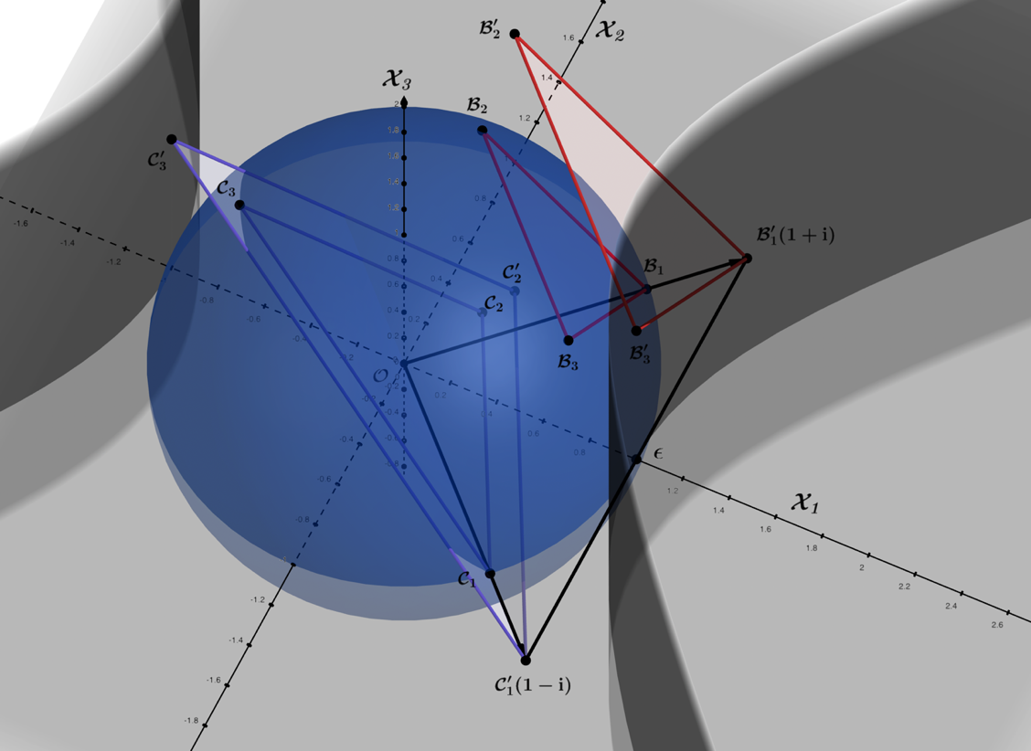
Figure 1.8.7 – Spher­i­cal and hy­per­bol­ic geome­tries in re­la­tion­ship to sym­met­ric as­ymp­tot­ic light Lie al­ge­bra gen­er­a­tors. ℬj,𝒞j\mathcal{B}_{j},\mathcal{C}_{j} rep­re­sent the gen­er­a­tors on the in­fi­nite sphere of tan­gent spaces, for ℬj′,𝒞j′=2( ℬj,𝒞j)\mathcal{B}'_{j},\mathcal{C}'_{j} = \sqrt{2}\left( \ \mathcal{B}_{j},\mathcal{C}_{j} \right).

The sym­met­ric as­ymp­tot­ic light Lie al­ge­bra gen­er­a­tors are de­pict­ed in Figure 1.8.7 as al­ge­bras on the unit sin­gu­lar­i­ty's sur­face (ℬj,𝒞j)\left( \mathcal{B}_{j},\mathcal{C}_{j} \right), and with their moduli ex­tend­ed to ℬj′,𝒞j′=2( ℬj,𝒞j)\mathcal{B}'_{j},\mathcal{C}'_{j} = \sqrt{2}\left( \ \mathcal{B}_{j},\mathcal{C}_{j} \right). For our energy-mo­men­tum ex­am­ple, we are using an X1X_{1}-type gen­er­a­tor, mean­ing the vec­tors ex­tend­ing to the poly­gon ver­tices at ℬj′,𝒞j′\mathcal{B}'_{j},\mathcal{C}'_{j} rep­re­sent the axes of ro­ta­tion. The point at ϵ\epsilon is a sig­nif­i­cant one, given that its lo­ca­tion rep­re­sents where spher­i­cal and hy­per­bol­ic geom­e­try share a common so­lu­tion, which for the eAχ,eiΩτe^{\mathrm{A}\chi},e^{i\Omega\tau} group gen­er­a­tors, occurs when χ,τ=0\chi,\tau = 0

eAχ(0)=eiΩτ(0)=cosh⁡(0)=cos⁡(0)=ϵ.\begin{array}{r} e^{\mathrm{A}\chi(0)} = e^{i\Omega\tau(0)} = \cosh(0) = \cos(0) = \epsilon. \end{array}
(1.8.165)

The 2\sqrt{2} factor is geo­met­ri­cal­ly the radial length of hy­potenuse formed by the tri­an­gle 𝒪ϵℬ1′ or the triangle 𝒪ϵC1′\mathcal{O}\epsilon\mathcal{B}_{1}^{'}\ \text{or the triangle}\ \mathcal{O}\epsilon C_{1}^{'}, and sig­ni­fies the point at which a seg­ment or­thog­o­nal to the X1X_{1}-axis will touch the light as­ymp­totes at ℬ1′\mathcal{B}_{1}^{'} and 𝒞1′\mathcal{C}_{1}^{'}. These points rep­re­sent the first in­ter­ac­tion points that as­ymp­tot­ic light has with space­time.

As pre­vi­ous­ly stated, net-zero is a char­ac­ter­is­tic that all physics must be con­sis­tent with, and the energy-mo­men­tum re­la­tion­ship is not an ex­cep­tion. For each XjX_{j}-plane, the light as­ymp­totes co­in­cid­ing with each of the four axes are so­lu­tions to the energy-mo­men­tum re­la­tion­ship, with two pos­i­tive so­lu­tions and two neg­a­tive. In our ex­am­ple case for the X1X_{1}-plane, the fol­low­ing light as­ymp­tote prod­ucts rep­re­sent the so­lu­tions to the geo­met­ric-de­pen­dent energy-mo­men­tum re­la­tion­ship**s for each of the four axes

E[X1]2=(m0c2(100001010)+pc(i0000i0i0))(m0c2(100001010)+pc(−i0000−i0−i0)),\begin{array}{r} \mathrm{E}_{\left\lbrack X_{1} \right\rbrack}^{2} = \left( m_{0}c^{2}\begin{pmatrix} 1 & 0 & 0 \\ 0 & 0 & 1 \\ 0 & 1 & 0 \end{pmatrix} + pc\begin{pmatrix} i & 0 & 0 \\ 0 & 0 & i \\ 0 & i & 0 \end{pmatrix} \right)\left( m_{0}c^{2}\begin{pmatrix} 1 & 0 & 0 \\ 0 & 0 & 1 \\ 0 & 1 & 0 \end{pmatrix} + pc\begin{pmatrix} - i & 0 & 0 \\ 0 & 0 & - i \\ 0 & - i & 0 \end{pmatrix} \right), \end{array}
(1.8.166)
E[iX1]2=(m0c2(−10000−10−10)+pc(i0000i0i0))(m0c2(100001010)+pc(i0000i0i0)),\begin{array}{r} \mathrm{E}_{\left\lbrack iX_{1} \right\rbrack}^{2} = \left( m_{0}c^{2}\begin{pmatrix} - 1 & 0 & 0 \\ 0 & 0 & - 1 \\ 0 & - 1 & 0 \end{pmatrix} + pc\begin{pmatrix} i & 0 & 0 \\ 0 & 0 & i \\ 0 & i & 0 \end{pmatrix} \right)\left( m_{0}c^{2}\begin{pmatrix} 1 & 0 & 0 \\ 0 & 0 & 1 \\ 0 & 1 & 0 \end{pmatrix} + pc\begin{pmatrix} i & 0 & 0 \\ 0 & 0 & i \\ 0 & i & 0 \end{pmatrix} \right), \end{array}
(1.8.167)
E[−X1]2=(m0c2(−10000−10−10)+pc(−i0000−i0−i0))(m0c2(−10000−10−10)+pc(i0000i0i0)),\begin{array}{r} \mathrm{E}_{\left\lbrack - X_{1} \right\rbrack}^{2} = \left( m_{0}c^{2}\begin{pmatrix} - 1 & 0 & 0 \\ 0 & 0 & - 1 \\ 0 & - 1 & 0 \end{pmatrix} + pc\begin{pmatrix} - i & 0 & 0 \\ 0 & 0 & - i \\ 0 & - i & 0 \end{pmatrix} \right)\left( m_{0}c^{2}\begin{pmatrix} - 1 & 0 & 0 \\ 0 & 0 & - 1 \\ 0 & - 1 & 0 \end{pmatrix} + pc\begin{pmatrix} i & 0 & 0 \\ 0 & 0 & i \\ 0 & i & 0 \end{pmatrix} \right), \end{array}
(1.8.168)
E[−iX1]2=(m0c2(100001010)+pc(−i0000−i0−i0))(m0c2(−10000−10−10)+pc(−i0000−i0−i0)),\begin{array}{r} \mathrm{E}_{\left\lbrack - iX_{1} \right\rbrack}^{2} = \left( m_{0}c^{2}\begin{pmatrix} 1 & 0 & 0 \\ 0 & 0 & 1 \\ 0 & 1 & 0 \end{pmatrix} + pc\begin{pmatrix} - i & 0 & 0 \\ 0 & 0 & - i \\ 0 & - i & 0 \end{pmatrix} \right)\left( m_{0}c^{2}\begin{pmatrix} - 1 & 0 & 0 \\ 0 & 0 & - 1 \\ 0 & - 1 & 0 \end{pmatrix} + pc\begin{pmatrix} - i & 0 & 0 \\ 0 & 0 & - i \\ 0 & - i & 0 \end{pmatrix} \right), \end{array}
(1.8.169)

where the sub­scripts for each E[cjX1]2\mathrm{E}_{\left\lbrack {c_{j}X}_{1} \right\rbrack}^{2} denote the axis. By ex­pand­ing each so­lu­tion, we find the re­sult­ing axis-de­pen­dent geo­met­ric-de­pen­dent energy-mo­men­tum**s

E[X1]2=(m02c4000m02c4000m02c4)+(p2c2000p2c2000p2c2),\begin{array}{r} \mathrm{E}_{\left\lbrack X_{1} \right\rbrack}^{2} = \begin{pmatrix} m_{0}^{2}c^{4} & 0 & 0 \\ 0 & m_{0}^{2}c^{4} & 0 \\ 0 & 0 & m_{0}^{2}c^{4} \end{pmatrix} + \begin{pmatrix} p^{2}c^{2} & 0 & 0 \\ 0 & p^{2}c^{2} & 0 \\ 0 & 0 & p^{2}c^{2} \end{pmatrix}, \end{array}
(1.8.170)
E[iXi]2=(−m02c4000−m02c4000−m02c4)+(−p2c2000−p2c2000−p2c2),\begin{array}{r} \mathrm{E}_{\left\lbrack {iX}_{i} \right\rbrack}^{2} = \begin{pmatrix} - m_{0}^{2}c^{4} & 0 & 0 \\ 0 & - m_{0}^{2}c^{4} & 0 \\ 0 & 0 & - m_{0}^{2}c^{4} \end{pmatrix} + \begin{pmatrix} - p^{2}c^{2} & 0 & 0 \\ 0 & - p^{2}c^{2} & 0 \\ 0 & 0 & - p^{2}c^{2} \end{pmatrix}, \end{array}
(1.8.171)
E[−X1]2=(m02c4000m02c4000m02c4)+(p2c2000p2c2000p2c2),\begin{array}{r} \mathrm{E}_{\left\lbrack {- X}_{1} \right\rbrack}^{2} = \begin{pmatrix} m_{0}^{2}c^{4} & 0 & 0 \\ 0 & m_{0}^{2}c^{4} & 0 \\ 0 & 0 & m_{0}^{2}c^{4} \end{pmatrix} + \begin{pmatrix} p^{2}c^{2} & 0 & 0 \\ 0 & p^{2}c^{2} & 0 \\ 0 & 0 & p^{2}c^{2} \end{pmatrix}, \end{array}
(1.8.172)
E[−iXi]2=(−m02c4000−m02c4000−m02c4)+(−p2c2000−p2c2000−p2c2),\begin{array}{r} \mathrm{E}_{\left\lbrack {- iX}_{i} \right\rbrack}^{2} = \begin{pmatrix} - m_{0}^{2}c^{4} & 0 & 0 \\ 0 & - m_{0}^{2}c^{4} & 0 \\ 0 & 0 & - m_{0}^{2}c^{4} \end{pmatrix} + \begin{pmatrix} - p^{2}c^{2} & 0 & 0 \\ 0 & - p^{2}c^{2} & 0 \\ 0 & 0 & - p^{2}c^{2} \end{pmatrix}, \end{array}
(1.8.173)

which, when summed, are equal to net-zero

∑E[cjX1]2=0.\begin{array}{r} \sum_{}^{}\mathrm{E}_{\left\lbrack {c_{j}X}_{1} \right\rbrack}^{2} = 0. \end{array}
(1.8.174)

The neg­a­tive-valued E[cjX1]2\mathrm{E}_{\left\lbrack {c_{j}X}_{1} \right\rbrack}^{2} energy-mo­men­tums are the result of the prod­uct of imag­i­nary-valued masses and mo­men­tums, which can be shown by start­ing with the neg­a­tive-valued re­sults for the imag­i­nary axes

E2=(−m02c4000−m02c4000−m02c4)+(−p2c2000−p2c2000−p2c2),\begin{array}{r} \mathrm{E}^{2} = \begin{pmatrix} - m_{0}^{2}c^{4} & 0 & 0 \\ 0 & - m_{0}^{2}c^{4} & 0 \\ 0 & 0 & - m_{0}^{2}c^{4} \end{pmatrix} + \begin{pmatrix} - p^{2}c^{2} & 0 & 0 \\ 0 & - p^{2}c^{2} & 0 \\ 0 & 0 & - p^{2}c^{2} \end{pmatrix}, \end{array}
(1.8.175)

and then solve for the energy E\mathrm{E}

E=−[(m02c4000m02c4000m02c4)+(p2c2000p2c2000p2c2)]\mathrm{E} = \sqrt{- \left\lbrack \begin{pmatrix} m_{0}^{2}c^{4} & 0 & 0 \\ 0 & m_{0}^{2}c^{4} & 0 \\ 0 & 0 & m_{0}^{2}c^{4} \end{pmatrix} + \begin{pmatrix} p^{2}c^{2} & 0 & 0 \\ 0 & p^{2}c^{2} & 0 \\ 0 & 0 & p^{2}c^{2} \end{pmatrix} \right\rbrack}
=i(m02c4000m02c4000m02c4)+(p2c2000p2c2000p2c2).\begin{array}{r} = i\sqrt{\begin{pmatrix} m_{0}^{2}c^{4} & 0 & 0 \\ 0 & m_{0}^{2}c^{4} & 0 \\ 0 & 0 & m_{0}^{2}c^{4} \end{pmatrix} + \begin{pmatrix} p^{2}c^{2} & 0 & 0 \\ 0 & p^{2}c^{2} & 0 \\ 0 & 0 & p^{2}c^{2} \end{pmatrix}}. \end{array}
(1.8.176)

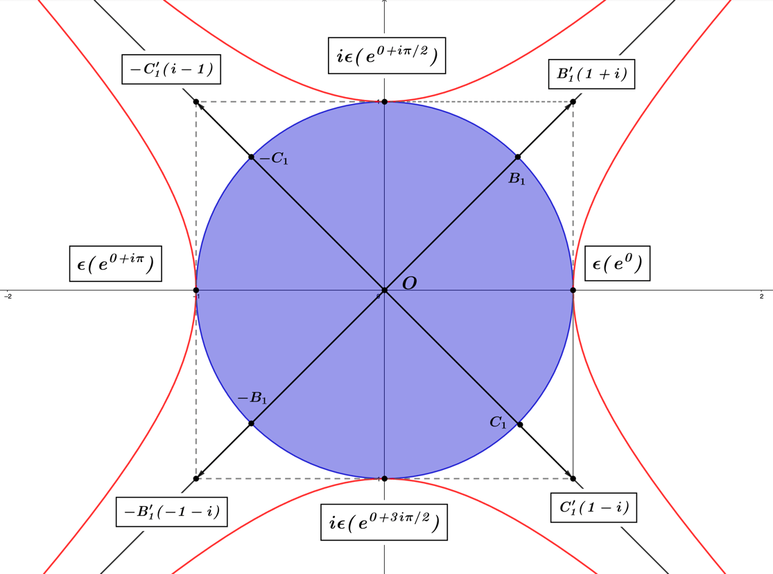
Figure 1.8.8 de­picts the geo­met­ric arrange­ment of the as­ymp­tot­ic light Lie al­ge­bra gen­er­a­tors in the X1X_{1}-plane. The points at the vector arrow tips form pairs with ad­ja­cent points on the light as­ymp­totes, rep­re­sent­ing the axes of the so­lu­tions to the geo­met­ric-de­pen­dent energy-mo­men­tum re­la­tion­ships. The dashed lines ex­tend­ing or­thog­o­nal­ly from each axis to the primed points on the light as­ymp­totes, present an in­tu­itive glimpse as to how Eu­clid­ean spaces man­i­fest in the Uni­fied Field, given the flat geom­e­try of the tri­an­gles formed with the axes where the Pythagore­an the­o­rem is ap­plic­a­ble. These primed points rep­re­sent the bal­ance points be­tween spher­i­cal and hy­per­bol­ic geom­e­try.

Figure
Figure 1.8.8 – A sym­met­ric slice of unit sin­gu­lar­i­ty through the origin rep­re­sent­ing the X1X_{1}-plane. The spher­i­cal and hy­per­bol­ic geome­tries are shown in re­la­tion­ship to sym­met­ric as­ymp­tot­ic light Lie al­ge­bra gen­er­a­tors.

The ad­ja­cent light as­ymp­totes form geo­met­ric prod­ucts that yield the ori­gins of the unit hy­per­bo­lae pic­tured in red in the figure

ℬ1×𝒞1=e(iπ4)e(−iπ4)=ϵ(e0),\mathcal{B}_{1} \times \mathcal{C}_{1} = e^{\left( \frac{i\pi}{4} \right)}e^{\left( - \frac{i\pi}{4} \right)} = \epsilon\left( e^{0} \right),
−𝒞1×ℬ1=e(i3π4)e(iπ4)=ϵ(eiπ),- \mathcal{C}_{1} \times \mathcal{B}_{1} = e^{\left( \frac{i3\pi}{4} \right)}e^{\left( \frac{i\pi}{4} \right)} = \epsilon\left( e^{i\pi} \right),
−ℬ1×−𝒞1=e(−3iπ4)e(3iπ4)=ϵ(e0),- \mathcal{B}_{1} \times - \mathcal{C}_{1} = e^{\left( - \frac{3i\pi}{4} \right)}e^{\left( \frac{3i\pi}{4} \right)} = \epsilon\left( e^{0} \right),
𝒞1×−ℬ1=e(−iπ4)e(−3iπ4)=ϵ(eiπ),\begin{array}{r} \mathcal{C}_{1} \times - \mathcal{B}_{1} = e^{\left( - \frac{i\pi}{4} \right)}e^{\left( - \frac{3i\pi}{4} \right)} = \epsilon\left( e^{i\pi} \right), \end{array}
(1.8.177)

where con­sis­tent with net-zero, we find sym­me­try in two pos­i­tive and neg­a­tive re­sult­ing pairs. The pos­i­tive-valued unit hy­per­bo­lae are ori­ent­ed in the space-like light cone, while the neg­a­tive-valued unit hy­per­bo­lae are ori­ent­ed in time-like light cone. The hy­per­bol­ic geome­tries in­her­ent in the Lie al­ge­bra gen­er­a­tors lo­cat­ed at these axis points can be ap­pre­ci­at­ed by start­ing with the fol­low­ing ℬ1(X1)\mathcal{B}_{1}\left( X_{1} \right) matrix Lie group gen­er­a­tor

ℬ1(X1)=exp⁡(iπ40000iπ40iπ40)=(eiπ4000cos⁡(π4)isin(π4)0isin(π4)cos⁡(π4)),\begin{array}{r} \mathcal{B}_{1}\left( X_{1} \right) = \exp\begin{pmatrix} \frac{i\pi}{4} & 0 & 0 \\ 0 & 0 & \frac{i\pi}{4} \\ 0 & \frac{i\pi}{4} & 0 \end{pmatrix} = \begin{pmatrix} e^{\frac{i\pi}{4}} & 0 & 0 \\ 0 & \cos\left( \frac{\pi}{4} \right) & isin\left( \frac{\pi}{4} \right) \\ 0 & isin\left( \frac{\pi}{4} \right) & \cos\left( \frac{\pi}{4} \right) \end{pmatrix}, \end{array}
(1.8.178)

which is equal to our geo­met­ric-de­pen­dent Schrödinger equa­tion wave­func­tion

ψ([A,Ω],[χ,τ])=(eαχ+iωτ000cos⁡(ωτ−iαχ)isin(ωτ−iαχ)0isin(ωτ−iαχ)cos⁡(ωτ−iαχ)),\begin{array}{r} \psi\left( \lbrack \mathrm{A},\Omega\rbrack,\lbrack\chi,\tau\rbrack \right) = \begin{pmatrix} e^{\alpha\chi + i\omega\tau} & 0 & 0 \\ 0 & \cos(\omega\tau - i\alpha\chi) & {isin}(\omega\tau - i\alpha\chi) \\ 0 & {isin}(\omega\tau - i\alpha\chi) & \cos(\omega\tau - i\alpha\chi) \end{pmatrix}, \end{array}
(1.8.179)

with its vari­ables set as ω=π4\omega = \frac{\pi}{4}, τ=1\tau = 1, and χ=0.\chi = 0.The group gen­er­a­tor can be ex­pressed in the equiv­a­lent form

ℬ1(X1)=((12+i2)00012i20i212),\begin{array}{r} \mathcal{B}_{1}\left( X_{1} \right) = \begin{pmatrix} \left( \frac{1}{\sqrt{2}} + \frac{i}{\sqrt{2}} \right) & 0 & 0 \\ 0 & \frac{1}{\sqrt{2}} & \frac{i}{\sqrt{2}} \\ 0 & \frac{i}{\sqrt{2}} & \frac{1}{\sqrt{2}} \end{pmatrix}, \end{array}
(1.8.180)

which shows its as­ymp­tot­ic light char­ac­ter­is­tics. ℬ1(X1)\mathcal{B}_{1}\left( X_{1} \right) is uni­tary given that

ℬ1(X1)×(ℬ1(X1))∗=ϵ,\begin{array}{r} \mathcal{B}_{1}\left( X_{1} \right) \times \left( \mathcal{B}_{1}\left( X_{1} \right) \right)^{*} = \epsilon, \end{array}
(1.8.181)

and sits on the bound­ary of the unit sin­gu­lar­i­ty. We can rotate the group in a clock­wise di­rec­tion to four equidis­tant points in ra­di­ans along the ge­o­des­ic path of the X1X_{1}-plane, by mul­ti­ply­ing suc­ces­sive­ly by −i- i. This leads to the fol­low­ing four dis­tinct as­ymp­tot­ic light group gen­er­a­tors

𝒞1(X1)=(−i)1×ℬ1(X1)=((12−i2)000−i212012−i2),\begin{array}{r} {{\mathcal{C}_{1}\left( X_{1} \right) = ( - i)}^{1}\times \mathcal{B}}_{1}\left( X_{1} \right) = \begin{pmatrix} \left( \frac{1}{\sqrt{2}} - \frac{i}{\sqrt{2}} \right) & 0 & 0 \\ 0 & - \frac{i}{\sqrt{2}} & \frac{1}{\sqrt{2}} \\ 0 & \frac{1}{\sqrt{2}} & - \frac{i}{\sqrt{2}} \end{pmatrix}, \end{array}
(1.8.182)
−ℬ1(X1)=(−i)2×ℬ1(X1)=((−12−i2)000−12−i20−i2−12),\begin{array}{r} - {{\mathcal{B}_{1}\left( X_{1} \right) = ( - i)}^{2}\times \mathcal{B}}_{1}\left( X_{1} \right) = \begin{pmatrix} \left( - \frac{1}{\sqrt{2}} - \frac{i}{\sqrt{2}} \right) & 0 & 0 \\ 0 & - \frac{1}{\sqrt{2}} & - \frac{i}{\sqrt{2}} \\ 0 & - \frac{i}{\sqrt{2}} & - \frac{1}{\sqrt{2}} \end{pmatrix}, \end{array}
(1.8.183)
−𝒞1(X1)=(−i)3×ℬ1(X1)=((−12+i2)000−12i20i2−12),\begin{array}{r} - {{\mathcal{C}_{1}\left( X_{1} \right) = ( - i)}^{3}\times \mathcal{B}}_{1}\left( X_{1} \right) = \begin{pmatrix} \left( - \frac{1}{\sqrt{2}} + \frac{i}{\sqrt{2}} \right) & 0 & 0 \\ 0 & - \frac{1}{\sqrt{2}} & \frac{i}{\sqrt{2}} \\ 0 & \frac{i}{\sqrt{2}} & - \frac{1}{\sqrt{2}} \end{pmatrix}, \end{array}
(1.8.184)
ℬ1(X1)=(−i)4×ℬ1(X1)=((12+i2)00012i20i212),\begin{array}{r} \mathcal{B}_{1}\left( X_{1} \right){{= ( - i)}^{4}\times \mathcal{B}}_{1}\left( X_{1} \right) = \begin{pmatrix} \left( \frac{1}{\sqrt{2}} + \frac{i}{\sqrt{2}} \right) & 0 & 0 \\ 0 & \frac{1}{\sqrt{2}} & \frac{i}{\sqrt{2}} \\ 0 & \frac{i}{\sqrt{2}} & \frac{1}{\sqrt{2}} \end{pmatrix}, \end{array}
(1.8.185)

and the com­plete ge­o­des­ic has been trav­elled given that (−i)4=ϵ( - i)^{4} = \epsilon, bring­ing us back to the start­ing group, ℬ1(X1)\mathcal{B}_{1}\left( X_{1} \right).

The prod­uct result of the light as­ymp­tote gen­er­a­tors ℬ1(X1)×𝒞1(X1)\mathcal{B}_{1}\left( X_{1} \right) \times \mathcal{C}_{1}\left( X_{1} \right) yields the hy­per­bol­ic Lie al­ge­bra gen­er­a­tor

ℬ1(X1)×𝒞1(X1)=(100001010),\begin{array}{r} \mathcal{B}_{1}\left( X_{1} \right) \times \mathcal{C}_{1}\left( X_{1} \right) = \begin{pmatrix} 1 & 0 & 0 \\ 0 & 0 & 1 \\ 0 & 1 & 0 \end{pmatrix}, \end{array}
(1.8.186)

which is a ro­ta­tor that acts on the X1X_{1}-plane hy­per­bol­ic gen­er­a­tor group

eA=(eα000cosh⁡(α)sinh⁡(α)0sinh⁡(α)cosh⁡(α)),\begin{array}{r} e^{\mathrm{A}} = \begin{pmatrix} e^{\alpha} & 0 & 0 \\ 0 & \cosh(\alpha) & \sinh(\alpha) \\ 0 & \sinh(\alpha) & \cosh(\alpha) \end{pmatrix}, \end{array}
(1.8.187)

taking the bottom-right 2×22 \times 2 sub­ma­trix from its hor­i­zon­tal ori­en­ta­tion to a ver­ti­cal one in the X1X_{1}-plane

eA(ℬ1(X1)×𝒞1(X1))=(eα000sinh⁡(α)cosh⁡(α)0cosh⁡(α)sinh⁡(α)),\begin{array}{r} e^{\mathrm{A}}\left( \mathcal{B}_{1}\left( X_{1} \right) \times \mathcal{C}_{1}\left( X_{1} \right) \right) = \begin{pmatrix} e^{\alpha} & 0 & 0 \\ 0 & \sinh(\alpha) & \cosh(\alpha) \\ 0 & \cosh(\alpha) & \sinh(\alpha) \end{pmatrix}, \end{array}
(1.8.188)

where it can be seen that cosh⁡(α)\cosh(\alpha) and sinh⁡(α)\sinh(\alpha) have been ex­changed. This result is con­sid­ered by math­e­mati­cians and physi­cists to be a linear trans­for­ma­tion con­sis­tent with the de­riv­a­tive rep­re­sen­ta­tion of the exp⁡(αℬ1(X1)×𝒞1(X1))\exp\left( \alpha\mathcal{B}_{1}\left( X_{1} \right) \times \mathcal{C}_{1}\left( X_{1} \right) \right) gen­er­a­tor, seen as

ddα[(eα000cosh⁡(α)sinh⁡(α)0sinh⁡(α)cosh⁡(α))]=(eα000sinh⁡(α)cosh⁡(α)0cosh⁡(α)sinh⁡(α)).\begin{array}{r} \frac{d}{d\alpha}\left\lbrack \begin{pmatrix} e^{\alpha} & 0 & 0 \\ 0 & \cosh(\alpha) & \sinh(\alpha) \\ 0 & \sinh(\alpha) & \cosh(\alpha) \end{pmatrix} \right\rbrack = \begin{pmatrix} e^{\alpha} & 0 & 0 \\ 0 & \sinh(\alpha) & \cosh(\alpha) \\ 0 & \cosh(\alpha) & \sinh(\alpha) \end{pmatrix}. \end{array}
(1.8.189)

Math­e­mat­i­cal­ly, the co­he­sive de­riv­a­tive of the above matrix is the result of our de­fined de­riv­a­tive op­er­a­tor trans­form

[(eα000cosh⁡(α)sinh⁡(α)0sinh⁡(α)cosh⁡(α))](ddα0000ddα0ddα0)=(eα000cosh⁡(α)sinh⁡(α)0sinh⁡(α)cosh⁡(α)),\begin{array}{r} \left\lbrack \begin{pmatrix} e^{\alpha} & 0 & 0 \\ 0 & \cosh(\alpha) & \sinh(\alpha) \\ 0 & \sinh(\alpha) & \cosh(\alpha) \end{pmatrix} \right\rbrack\begin{pmatrix} \frac{d}{d\alpha} & 0 & 0 \\ 0 & 0 & \frac{d}{d\alpha} \\ 0 & \frac{d}{d\alpha} & 0 \end{pmatrix} = \begin{pmatrix} e^{\alpha} & 0 & 0 \\ 0 & \cosh(\alpha) & \sinh(\alpha) \\ 0 & \sinh(\alpha) & \cosh(\alpha) \end{pmatrix}, \end{array}
(1.8.190)

which is con­sis­tent with the result of the de­riv­a­tive of the ex­po­nen­tial func­tion

ddα[eα]=eα.\begin{array}{r} \frac{d}{d\alpha}\left\lbrack e^{\alpha} \right\rbrack = e^{\alpha}. \end{array}
(1.8.191)

When the ℬ1(X1)×𝒞1(X1)\mathcal{B}_{1}\left( X_{1} \right) \times \mathcal{C}_{1}\left( X_{1} \right) light as­ymp­tote ro­ta­tor acts on eA(ℬ1(X1)×𝒞1(X1))e^{\mathrm{A}}\left( \mathcal{B}_{1}\left( X_{1} \right) \times \mathcal{C}_{1}\left( X_{1} \right) \right), it re­turns to its orig­i­nal po­si­tion

eA(ℬ1(X1)×𝒞1(X1))2=(eα000cosh⁡(α)sinh⁡(α)0sinh⁡(α)cosh⁡(α))=eA,\begin{array}{r} e^{\mathrm{A}}\left( \mathcal{B}_{1}\left( X_{1} \right) \times \mathcal{C}_{1}\left( X_{1} \right) \right)^{2} = \begin{pmatrix} e^{\alpha} & 0 & 0 \\ 0 & \cosh(\alpha) & \sinh(\alpha) \\ 0 & \sinh(\alpha) & \cosh(\alpha) \end{pmatrix} = e^{\mathrm{A}}, \end{array}
(1.8.192)

given that the ro­ta­tor squares to the iden­ti­ty matrix

(ℬ1(X1)×𝒞1(X1))2=(100001010)2=(100010001),\begin{array}{r} \left( \mathcal{B}_{1}\left( X_{1} \right) \times \mathcal{C}_{1}\left( X_{1} \right) \right)^{2} = \begin{pmatrix} 1 & 0 & 0 \\ 0 & 0 & 1 \\ 0 & 1 & 0 \end{pmatrix}^{2} = \begin{pmatrix} 1 & 0 & 0 \\ 0 & 1 & 0 \\ 0 & 0 & 1 \end{pmatrix}, \end{array}
(1.8.193)

which gives rise to an ori­ent­ed geo­met­ric con­fine­ment these hy­per­bol­ic gen­er­a­tors main­tain be­tween the pos­i­tive ver­ti­cal and hor­i­zon­tal axes in the X1X_{1}-plane. Eval­u­a­tion of the de­ter­mi­nants for the two Lie group gen­er­a­tors yields the fol­low­ing re­sults

det⁡(eA)=eα(cosh2⁡(α)−sinh2⁡(α))=eα,\begin{array}{r} \det\left( e^{\mathrm{A}} \right) = e^{\alpha}\left( \cosh^{2}{(\alpha) - \sinh^{2}(\alpha)} \right) = e^{\alpha}, \end{array}
(1.8.194)
det⁡(eA(ℬ1(X1)×𝒞1(X1)))=eα(sinh2⁡(α)−cosh2⁡(α))=−eα,\begin{array}{r} \det\left( e^{\mathrm{A}}\left( \mathcal{B}_{1}\left( X_{1} \right) \times \mathcal{C}_{1}\left( X_{1} \right) \right) \right) = e^{\alpha}\left( \sinh^{2}{(\alpha) - \cosh^{2}(\alpha)} \right) = {- e}^{\alpha}, \end{array}
(1.8.195)

where the first rep­re­sents the space-like geom­e­try of the unit hy­per­bo­la ori­ent­ed in the hor­i­zon­tal pos­i­tive real-axis, and the second rep­re­sents the time-like geom­e­try of the unit hy­per­bo­la ori­ent­ed in the ver­ti­cal real-axis.

As­sum­ing the pre­vi­ous ex­am­ple was form, the hy­per­bol­ic analog anti-form is the result of the prod­uct of the −𝒞1(X1)- \mathcal{C}_{1}\left( X_{1} \right) and −ℬ1(X1)- \mathcal{B}_{1}\left( X_{1} \right) light as­ymp­totes

−𝒞1(X1)×−ℬ1(X1)=(100001010),\begin{array}{r} - \mathcal{C}_{1}\left( X_{1} \right) \times - \mathcal{B}_{1}\left( X_{1} \right) = \begin{pmatrix} 1 & 0 & 0 \\ 0 & 0 & 1 \\ 0 & 1 & 0 \end{pmatrix}, \end{array}
(1.8.196)

which is the ro­ta­tor that acts on the hy­per­bol­ic gen­er­a­tor group in the neg­a­tive X1X_{1}-plane

e−A=(e−α000cosh⁡(α)−sinh(α)0−sinh(α)cosh⁡(α)),\begin{array}{r} e^{- \mathrm{A}} = \begin{pmatrix} e^{- \alpha} & 0 & 0 \\ 0 & \cosh(\alpha) & {- sinh}(\alpha) \\ 0 & {- sinh}(\alpha) & \cosh(\alpha) \end{pmatrix}, \end{array}
(1.8.197)

taking the bottom-right 2×22 \times 2 sub­ma­trix in the neg­a­tive X1X_{1}-plane from its hor­i­zon­tal ori­en­ta­tion to a ver­ti­cal one

e−A(−𝒞1(X1)×−ℬ1(X1))=(e−α000−sinh(α)cosh⁡(α)0cosh⁡(α)−sinh(α)),\begin{array}{r} e^{- \mathrm{A}}\left( - \mathcal{C}_{1}\left( X_{1} \right) \times - \mathcal{B}_{1}\left( X_{1} \right) \right) = \begin{pmatrix} e^{- \alpha} & 0 & 0 \\ 0 & {- sinh}(\alpha) & \cosh(\alpha) \\ 0 & \cosh(\alpha) & {- sinh}(\alpha) \end{pmatrix}, \end{array}
(1.8.198)

where it can be seen that cosh⁡(α)\cosh(\alpha) and −sinh(α){- sinh}(\alpha) func­tions have been ex­changed. A sim­i­lar­ly ori­ent­ed geo­met­ric anti-form con­fine­ment is also present due to the second prod­uct power equal­ing the iden­ti­ty

(−𝒞1(X1)×−ℬ1(X1))2=(100010001),\begin{array}{r} \left( - \mathcal{C}_{1}\left( X_{1} \right) \times - \mathcal{B}_{1}\left( X_{1} \right) \right)^{2} = \begin{pmatrix} 1 & 0 & 0 \\ 0 & 1 & 0 \\ 0 & 0 & 1 \end{pmatrix}, \end{array}
(1.8.199)

and these hy­per­bol­ic gen­er­a­tors main­tain lo­ca­tions be­tween the neg­a­tive ver­ti­cal and hor­i­zon­tal axes in the X1X_{1}-plane. Eval­u­a­tion of the anti-form de­ter­mi­nants for these two Lie group gen­er­a­tors yields the fol­low­ing re­sults

det⁡(e−A)=e−α(cosh2⁡(α)−sinh2⁡(α))=e−α,\begin{array}{r} \det\left( e^{- \mathrm{A}} \right) = e^{- \alpha}\left( \cosh^{2}{(\alpha) - \sinh^{2}(\alpha)} \right) = e^{- \alpha}, \end{array}
(1.8.200)
det⁡(e−A(−𝒞1(X1)×−ℬ1(X1)))=e−α(sinh2⁡(α)−cosh2⁡(α))=−e−α,\begin{array}{r} \det\left( e^{- \mathrm{A}}\left( - \mathcal{C}_{1}\left( X_{1} \right) \times - \mathcal{B}_{1}\left( X_{1} \right) \right) \right) = e^{- \alpha}\left( \sinh^{2}{(\alpha) - \cosh^{2}(\alpha)} \right) = {- e}^{- \alpha}, \end{array}
(1.8.201)

where the first rep­re­sents the anti-space-like geom­e­try of the unit hy­per­bo­la ori­ent­ed in the hor­i­zon­tal neg­a­tive real-axis, and the second rep­re­sents the anti-time-like geom­e­try of the unit hy­per­bo­la ori­ent­ed in the ver­ti­cal neg­a­tive real-axis.

The pro­found im­pli­ca­tion is that time flows in one di­rec­tion for form, which is due to the geo­met­ric con­fine­ment its hy­per­bol­ic gen­er­a­tors are sub­ject to on the pos­i­tive real ver­ti­cal and hor­i­zon­tal axes. Anti-form trav­els in time in the op­po­site di­rec­tion with in­verse­ly re­lat­ed mag­ni­tudes for anti-time and anti-space com­pared to the time and space of forms. Time travel for some­thing bound to the geome­tries of form and anti-form, if pos­si­ble, re­quires the trans­for­ma­tion of form to anti-form and vice versa.

Geo­met­ri­cal­ly, mul­ti­ply­ing the ℬ1(X1)\mathcal{B}_{1}\left( X_{1} \right) group gen­er­a­tor by −i- i, ro­tates it by −π2- \frac{\pi}{2} ra­di­ans in the X1X_{1}-plane on the unit sin­gu­lar­i­ty. This ro­ta­tion is ex­act­ly what the −i- i term does to the wave­func­tion ψ(X,τ)\psi(X,\tau) on the left-hand side of the Schrödinger equa­tion

−iℏ∂∂τψ(X,τ)=[ℏ22m∂2∂X2+V(X,τ)]ψ(X,τ),\begin{array}{r} - i\hslash\frac{\partial}{\partial\tau}\psi(X,\tau) = \left\lbrack \frac{\hslash^{2}}{2m}\frac{\partial^{2}}{\partial X^{2}} + V(X,\tau) \right\rbrack\psi(X,\tau), \end{array}
(1.8.202)

and mul­ti­ply­ing by ii for the Schrödinger equa­tion of the form

iℏ∂∂τψ(X,τ)=[−ℏ22m∂2∂X2+V(X,τ)]ψ(X,τ),\begin{array}{r} i\hslash\frac{\partial}{\partial\tau}\psi(X,\tau) = \left\lbrack - \frac{\hslash^{2}}{2m}\frac{\partial^{2}}{\partial X^{2}} + V(X,\tau) \right\rbrack\psi(X,\tau), \end{array}
(1.8.203)

ro­tates ψ(X,τ)\psi(X,\tau) by π2\frac{\pi}{2} ra­di­ans in the X1X_{1}-plane on the unit sin­gu­lar­i­ty. The −π2- \frac{\pi}{2} ra­di­ans ro­ta­tion ap­plies just the same for the geo­met­ric-de­pen­dent Schrödinger equa­tion

−iℏψ([A,Ω],[χ,τ])∂τˆ=ℏ22mψ([A,Ω],[χ,τ])∂χ2ˆ,\begin{array}{r} - i\hslash\psi\left( \lbrack \mathrm{A},\Omega\rbrack,\lbrack\chi,\tau\rbrack \right)\widehat{\partial\tau} = \frac{\hslash^{2}}{2m}\psi\left( \lbrack \mathrm{A},\Omega\rbrack,\lbrack\chi,\tau\rbrack \right)\widehat{\partial\chi^{2}}, \end{array}
(1.8.204)

and the vari­able spe­cif­ic ψ([A,Ω],[χ,τ])\psi\left( \lbrack \mathrm{A},\Omega\rbrack,\lbrack\chi,\tau\rbrack \right) func­tion, that is the ℬ1(X1)\mathcal{B}_{1}\left( X_{1} \right) gen­er­a­tor.

Using our ψ([A,Ω],[χ,τ])\psi\left( \lbrack \mathrm{A},\Omega\rbrack,\lbrack\chi,\tau\rbrack \right) wave­func­tion, we omit the ℏ\hslash and ℏ2(2m)\frac{\hslash^{2}}{(2m)} terms in the geo­met­ric-de­pen­dent Schrödinger equa­tion, and eval­u­ate the equal­i­ty

−iψ([A,Ω],[χ,τ])∂τˆ=ψ([A,Ω],[χ,τ])∂χ2ˆ,\begin{array}{r} - i\psi\left( \lbrack \mathrm{A},\Omega\rbrack,\lbrack\chi,\tau\rbrack \right)\widehat{\partial\tau} = \psi\left( \lbrack \mathrm{A},\Omega\rbrack,\lbrack\chi,\tau\rbrack \right)\widehat{\partial\chi^{2}}, \end{array}
(1.8.205)

find­ing for the left-hand side

−iψ([A,Ω],[χ,τ])∂τˆ=ω(eαχ+iωτ000cos⁡(ωτ−iαχ)isin(ωτ−iαχ)0isin(ωτ−iαχ)cos⁡(ωτ−iαχ)),\begin{array}{r} - i\psi\left( \lbrack \mathrm{A},\Omega\rbrack,\lbrack\chi,\tau\rbrack \right)\widehat{\partial\tau} = \omega\begin{pmatrix} e^{\alpha\chi + i\omega\tau} & 0 & 0 \\ 0 & \cos(\omega\tau - i\alpha\chi) & {isin}(\omega\tau - i\alpha\chi) \\ 0 & {isin}(\omega\tau - i\alpha\chi) & \cos(\omega\tau - i\alpha\chi) \end{pmatrix}, \end{array}
(1.8.206)

then the right-hand side

ψ([A,Ω],[χ,τ])∂χ2ˆ=α2(eαχ+iωτ000cos⁡(ωτ−iαχ)sin⁡(ωτ−iαχ)0sin⁡(ωτ−iαχ)cos⁡(ωτ−iαχ)),\begin{array}{r} \psi\left( \lbrack \mathrm{A},\Omega\rbrack,\lbrack\chi,\tau\rbrack \right)\widehat{\partial\chi^{2}} = \alpha^{2}\begin{pmatrix} e^{\alpha\chi + i\omega\tau} & 0 & 0 \\ 0 & \cos(\omega\tau - i\alpha\chi) & \sin(\omega\tau - i\alpha\chi) \\ 0 & \sin(\omega\tau - i\alpha\chi) & \cos(\omega\tau - i\alpha\chi) \end{pmatrix}, \end{array}
(1.8.207)

and since the wave­func­tion ψ([A,Ω],[χ,τ])\psi\left( \lbrack \mathrm{A},\Omega\rbrack,\lbrack\chi,\tau\rbrack \right) is common to both re­sults, our equal­i­ty sim­pli­fies to

ω=α2.\begin{array}{r} \omega = \alpha^{2}. \end{array}
(1.8.208)

We recall that α\alpha is the wavenum­ber, and for matter waves, this equals

α=pℏ=2mEℏ,\begin{array}{r} \alpha = \frac{p}{\hslash} = \frac{\sqrt{2mE}}{\hslash}, \end{array}
(1.8.209)

and α2\alpha^{2} is

α2=2mEℏ2,\begin{array}{r} \alpha^{2} = \frac{2mE}{\hslash^{2}}, \end{array}
(1.8.210)

which, by using the energy equal­i­ty E=ℏωE = \hslash\omega, it can be put in terms of ω\omega as

α2=ω(2mℏ).\begin{array}{r} \alpha^{2} = \omega\left( \frac{2m}{\hslash} \right). \end{array}
(1.8.211)

There­fore, the geo­met­ric-de­pen­dent Schrödinger equa­tion for mas­sive body sys­tems is con­tin­u­al­ly solv­ing for the mass term mm, which is the sole in­de­pen­dent vari­able given that the an­gu­lar fre­quen­cy ω\omega and the wavenum­ber α\alpha are re­lat­ed by the iden­ti­ty

α=ωv,\begin{array}{r} \alpha = \omega v, \end{array}
(1.8.212)

where vv is the ve­loc­i­ty term, im­ply­ing that

2mℏ=ωv2.\begin{array}{r} \frac{2m}{\hslash} = \omega v^{2}. \end{array}
(1.8.213)

Solv­ing for the mass term in the α2\alpha^{2} ex­pres­sion, we find

α2=ω(2mℏ)→m=α2ℏω,\begin{array}{r} \alpha^{2} = \omega\left( \frac{2m}{\hslash} \right) \rightarrow m = \frac{\alpha^{2}\hslash}{\omega}, \end{array}
(1.8.214)

and by p=ℏαp = \hslash\alpha, the mass of the system is equal to

m=αω(ℏα)→αω(p),\begin{array}{r} m = \frac{\alpha}{\omega}(\hslash\alpha) \rightarrow \frac{\alpha}{\omega}(p), \end{array}
(1.8.215)

where the αω\frac{\alpha}{\omega} term above is equal to the in­verse of the ve­loc­i­ty

αω=ααv=1v,\begin{array}{r} \frac{\alpha}{\omega} = \frac{\alpha}{\alpha v} = \frac{1}{v}, \end{array}
(1.8.216)

which leads to the well-known mo­men­tum ex­pres­sion

m=pv→p=mv.\begin{array}{r} m = \frac{p}{v} \rightarrow p = mv. \end{array}
(1.8.217)

For the wave­func­tion ψ([A,Ω],[χ,τ])\psi\left( \lbrack \mathrm{A},\Omega\rbrack,\lbrack\chi,\tau\rbrack \right), the α\alpha and ω\omega vari­able terms will be equal in mag­ni­tude, and by as­sign­ing a vari­able θα=α\theta_{\alpha} = \alpha, and θω=ω\theta_{\omega} = \omega the wave­func­tion be­comes

ψ([Θ],[χ,τ])=(eθαχ+iθωτ000cos⁡(θωτ−iθαχ)sin⁡(θωτ−iθαχ)0sin⁡(θωτ−iθαχ)cos⁡(θωτ−iθαχ)).\begin{array}{r} \psi\left( \lbrack\Theta\rbrack,\lbrack\chi,\tau\rbrack \right) = \begin{pmatrix} e^{\theta_{\alpha}\chi + i\theta_{\omega}\tau} & 0 & 0 \\ 0 & \cos\left( \theta_{\omega}\tau - i\theta_{\alpha}\chi \right) & \sin\left( \theta_{\omega}\tau - i\theta_{\alpha}\chi \right) \\ 0 & \sin\left( \theta_{\omega}\tau - i\theta_{\alpha}\chi \right) & \cos\left( \theta_{\omega}\tau - i\theta_{\alpha}\chi \right) \end{pmatrix}. \end{array}
(1.8.218)

Using ψ([Θ],[χ,τ])\psi\left( \lbrack\Theta\rbrack,\lbrack\chi,\tau\rbrack \right), we eval­u­ate the equal­i­ty

−iψ([Θ],[χ,τ])∂τˆ=Kψ([Θ],[χ,τ])∂χ2ˆ,\begin{array}{r} - i\psi\left( \lbrack\Theta\rbrack,\lbrack\chi,\tau\rbrack \right)\widehat{\partial\tau} = \mathrm{K}\psi\left( \lbrack\Theta\rbrack,\lbrack\chi,\tau\rbrack \right)\widehat{\partial\chi^{2}}, \end{array}
(1.8.219)

for a vari­able, K\mathrm{K}, find­ing for the left-hand side

−iψ([Θ],[χ,τ])∂τˆ=θω(eθαχ+iθωτ000cos⁡(θωτ−iθαχ)sin⁡(θωτ−iθαχ)0sin⁡(θωτ−iθαχ)cos⁡(θωτ−iθαχ)),\begin{array}{r} - i\psi\left( \lbrack\Theta\rbrack,\lbrack\chi,\tau\rbrack \right)\widehat{\partial\tau} = \theta_{\omega}\begin{pmatrix} e^{\theta_{\alpha}\chi + i\theta_{\omega}\tau} & 0 & 0 \\ 0 & \cos\left( \theta_{\omega}\tau - i\theta_{\alpha}\chi \right) & \sin\left( \theta_{\omega}\tau - i\theta_{\alpha}\chi \right) \\ 0 & \sin\left( \theta_{\omega}\tau - i\theta_{\alpha}\chi \right) & \cos\left( \theta_{\omega}\tau - i\theta_{\alpha}\chi \right) \end{pmatrix}, \end{array}
(1.8.220)

then the right-hand side

Kψ([Θ],[χ,τ])∂χ2ˆ=θα2(eθαχ+iθωτ000cos⁡(θωτ−iθαχ)sin⁡(θωτ−iθαχ)0sin⁡(θωτ−iθαχ)cos⁡(θωτ−iθαχ)),\begin{array}{r} \mathrm{K}\psi\left( \lbrack\Theta\rbrack,\lbrack\chi,\tau\rbrack \right)\widehat{\partial\chi^{2}} = \theta_{\alpha}^{2}\begin{pmatrix} e^{\theta_{\alpha}\chi + i\theta_{\omega}\tau} & 0 & 0 \\ 0 & \cos\left( \theta_{\omega}\tau - i\theta_{\alpha}\chi \right) & \sin\left( \theta_{\omega}\tau - i\theta_{\alpha}\chi \right) \\ 0 & \sin\left( \theta_{\omega}\tau - i\theta_{\alpha}\chi \right) & \cos\left( \theta_{\omega}\tau - i\theta_{\alpha}\chi \right) \end{pmatrix}, \end{array}
(1.8.221)

and the equal­i­ty sim­pli­fies to

θω=Kθα2.\begin{array}{r} \theta_{\omega} = K\theta_{\alpha}^{2}. \end{array}
(1.8.222)

Using sim­i­lar vari­ables to the ℬ1(X1)\mathcal{B}_{1}\left( X_{1} \right) matrix Lie group gen­er­a­tor, we set θω,θα=π4\theta_{\omega},\theta_{\alpha} = \frac{\pi}{4}, and solve for the value of the fre­quen­cy

θω=π4=2πf→=18,\begin{array}{r} \theta_{\omega} = \frac{\pi}{4} = 2\pi f \rightarrow = \frac{1}{8}, \end{array}
(1.8.223)

and for the wave­length value

θα=π4=2πλ→λ=8.\begin{array}{r} \theta_{\alpha} = \frac{\pi}{4} = \frac{2\pi}{\lambda} \rightarrow \lambda = 8. \end{array}
(1.8.224)

We re­arrange the equal­i­ty

θω=θα2K→θωθα=θαK,\begin{array}{r} \theta_{\omega} = \theta_{\alpha}^{2}\mathrm{K} \rightarrow \frac{\theta_{\omega}}{\theta_{\alpha}} = \theta_{\alpha}\mathrm{K}, \end{array}
(1.8.225)

and given that

θωθα=c=1,\begin{array}{r} \frac{\theta_{\omega}}{\theta_{\alpha}} = c = 1, \end{array}
(1.8.226)

the ex­pres­sion be­comes

c=θαK.\begin{array}{r} c = \theta_{\alpha}\mathrm{K}. \end{array}
(1.8.227)

The ob­vi­ous so­lu­tion for K\mathrm{K} is

K=θωθα2,\begin{array}{r} K = \frac{\theta_{\omega}}{\theta_{\alpha}^{2}}, \end{array}
(1.8.228)

but the other so­lu­tion that exists for light is less ap­par­ent, which is seen by con­sid­er­ing K\mathrm{K} as

K=1θω,\begin{array}{r} \mathrm{K} = \frac{1}{\theta_{\omega}}, \end{array}
(1.8.229)

where the equal­i­ty be­comes

θωθα=θαK→2πf(2πλ)=(2πλ)2πf,\begin{array}{r} \frac{\theta_{\omega}}{\theta_{\alpha}} = \theta_{\alpha}\mathrm{K} \rightarrow \frac{2\pi f}{\left( \frac{2\pi}{\lambda} \right)} = \frac{\left( \frac{2\pi}{\lambda} \right)}{2\pi f}, \end{array}
(1.8.230)

which sim­pli­fies to

θωθα=θαK→fλ=1fλ.\begin{array}{r} \frac{\theta_{\omega}}{\theta_{\alpha}} = \theta_{\alpha}\mathrm{K} \rightarrow f\lambda = \frac{1}{f\lambda}. \end{array}
(1.8.231)

Above, we find an in­verse speed of light re­la­tion­ship that hold when c=fλ=1c = f\lambda = 1, which is ex­act­ly the case for our light system, ev­i­denced by sub­sti­tut­ing our fre­quen­cy and wavenum­ber values into the ex­pres­sion

fλ=1fλ→(18)(8)=1(18)(8)→1=1.\begin{array}{r} f\lambda = \frac{1}{f\lambda} \rightarrow \left( \frac{1}{8} \right)(8) = \frac{1}{\left( \frac{1}{8} \right)(8)} \rightarrow 1 = 1. \end{array}
(1.8.232)

Per­haps this is sur­pris­ing, but it is rooted in the es­sen­tial net-zero char­ac­ter­is­tics that light must pos­sess, mean­ing a light anti-form exists that is in­verse­ly re­lat­ed to its light-form coun­ter­part, which to­geth­er embody a per­fect bal­ance.

More ev­i­dence for the ex­is­tence of this bal­ance is ap­pre­ci­at­ed by eval­u­at­ing our light-system equal­i­ty using the matter-based ex­pres­sion for our wavenum­ber

θα=2mEℏ,\begin{array}{r} \theta_{\alpha} = \frac{\sqrt{2mE}}{\hslash}, \end{array}
(1.8.233)

which would be blas­phe­mous to the physi­cist, but the math­e­mat­ics clear­ly states oth­er­wise.

θα2=2mEℏ=θω(2mℏ),\begin{array}{r} \theta_{\alpha}^{2} = \frac{2mE}{\hslash} = \theta_{\omega}\left( \frac{2m}{\hslash} \right), \end{array}
(1.8.234)

Solv­ing for mass we find

m=θα2(ℏ2θω),\begin{array}{r} m = \theta_{\alpha}^{2}\left( \frac{\hslash}{2\theta_{\omega}} \right), \end{array}
(1.8.235)

and given that θα=θω\theta_{\alpha} = \theta_{\omega}, mass for the light system has two so­lu­tions

m=θωℏ2=θαℏ2.\begin{array}{r} m = \frac{\theta_{\omega}\hslash}{2} = \frac{\theta_{\alpha}\hslash}{2}. \end{array}
(1.8.236)

These can be ex­pressed in re­la­tion to a wave­length mass, mλ,m_{\lambda},and a fre­quen­cy mass, mω,m_{\omega},as

mf=2πfℏ2=fh2,\begin{array}{r} m_{f} = \frac{2\pi f\hslash}{2} = \frac{fh}{2}, \end{array}
(1.8.237)
mλ=2πℏ2λ=h2λ,\begin{array}{r} m_{\lambda} = \frac{2\pi\hslash}{2\lambda} = \frac{h}{2\lambda}, \end{array}
(1.8.238)

where mfm_{f} and mλm_{\lambda} are equal. This equiv­a­lence

mf=mλ→fh2=h2λ,\begin{array}{r} m_{f} = m_{\lambda} \rightarrow \frac{fh}{2} = \frac{h}{2\lambda}, \end{array}
(1.8.239)

can be arranged in two ratios: the first

mfmλ=(fh2)(h2λ)=2hfλ2h=fλ=c,\begin{array}{r} \frac{m_{f}}{m_{\lambda}} = \frac{\left( \frac{fh}{2} \right)}{\left( \frac{h}{2\lambda} \right)} = \frac{2hf\lambda}{2h} = f\lambda = c, \end{array}
(1.8.240)

and the second

mλmω=(h2λ)(fh2)=2h2hfλ=1fλ=1c,\begin{array}{r} \frac{m_{\lambda}}{m_{\omega}} = \frac{\left( \frac{h}{2\lambda} \right)}{\left( \frac{fh}{2} \right)} = \frac{2h}{2hf\lambda} = \frac{1}{f\lambda} = \frac{1}{c}, \end{array}
(1.8.241)

which are in­verse­ly re­lat­ed to one an­oth­er, yet equal in light sys­tems, and are indeed form and anti-form matter com­po­nents of light sys­tems. Set­ting the form and anti-form matter ratios as equal, we find

mfmλ=mλmω→fλ=1fλ→c=1c,\begin{array}{r} \frac{m_{f}}{m_{\lambda}} = \frac{m_{\lambda}}{m_{\omega}} \rightarrow f\lambda = \frac{1}{f\lambda} \rightarrow c = \frac{1}{c}, \end{array}
(1.8.242)

rep­re­sent­ing the same so­lu­tions found for K=1θω\mathrm{K} = \frac{1}{\theta_{\omega}}, in the ex­pres­sion

θωθα=θαK→θωθα=θαθω→fλ=1fλ→c=1c.\begin{array}{r} \frac{\theta_{\omega}}{\theta_{\alpha}} = \theta_{\alpha}\mathrm{K} \rightarrow \frac{\theta_{\omega}}{\theta_{\alpha}} = \frac{\theta_{\alpha}}{\theta_{\omega}} \rightarrow f\lambda = \frac{1}{f\lambda} \rightarrow c = \frac{1}{c}. \end{array}
(1.8.243)

As­ymp­tot­ic light is a bal­ance be­tween in­verse­ly re­lat­ed wave­lengths and fre­quen­cies, matter and in­verse matter, oth­er­wise known as matter and an­ti­mat­ter, form and anti-form. This brings us to the sub­ject matter of the next sec­tion, which is to math­e­mat­i­cal­ly ex­plore in­vari­ant mass and derive the as­so­ci­a­tion that a unit in­vari­ant mass has with the energy-mo­men­tum re­la­tion­ship.