1.3.4 Curvature

At the onset of this chapter, we discussed the positive curvature of the sphere, having the triangle angle the sum $> \pi$ , and the negative curvature of the pseudosphere, having an angle sum $< \pi$ . The term curvature can be thought of as the degree of deviation a curve has compared to the straight line, or the amount of deviation a surface has from that of the plane. Analytic functions are infinitely differentiable, and for some analytic function $f(t)$ the existence of $f^{'}(t),f^{''}(t)$ is guaranteed. Concerning a space parametrization, we can define $\gamma(s)$ , as

\begin{array}{r} \gamma(s) = \left( x(s),y(s) \right), \end{array}

(1.3.23)

and consider an analytic Euclidean function's arc segment distance, as

\begin{array}{r} \left\| \gamma^{'}(s) \right\| = \sqrt{x^{'}(s)^{2} + y^{'}(s)^{2}} = 1. \end{array}

(1.3.24)

The unit tangent vector $T(s)$ can then be defined in terms of $\gamma(s)$

\begin{array}{r} T(s) = \gamma^{'}(s) = \left( x^{'}(s),y'(s) \right), \end{array}

(1.3.25)

and a unit normal vector (orthogonal) to the curve is found by taking $T'(s)$

\begin{array}{r} T^{'}(s) = \left( x^{''}(s),y^{''}(s) \right). \end{array}

(1.3.26)

Curvature $\kappa$ can now be defined as the two-norm of the unit normal vector $T'(s)$

\begin{array}{r} \kappa = \left\| T^{'}(s) \right\| = \left\| \gamma^{''}(s) \right\| = \sqrt{x^{''}(s)^{2} + y^{''}(s)^{2}}, \end{array}

(1.3.27)

and the radius of curvature $R$ is then defined by the inverse relationship

\begin{array}{r} R = \frac{1}{\kappa}. \end{array}

(1.3.28)

$R$ will be equal to the radius of a circular arc at the point being evaluated on the curve. The signed curvature $k(s)$ is defined, as

\begin{array}{r} k(s) = \pm \kappa(s), \end{array}

(1.3.29)

and for a unit normal vector $\widehat{n}(s)$ oriented $\frac{i\pi}{2}$ radians counterclockwise to $T(s)$ , $k(s)$ relates to $T^{'}(s)$ by the following expression

\begin{array}{r} T^{'}(s) = k(s)\widehat{n}(s). \end{array}

(1.3.30)

Using the parameterization $\gamma(s) = \left( x(s),y(s) \right)$ , the calculation for signed curvature is

\begin{array}{r} k = \frac{x^{'}y^{''} - y^{'}x^{''}}{\left( x^{'2} + y^{'2} \right)^{\frac{3}{2}}}, \end{array}

(1.3.31)

and for curvature

\begin{array}{r} \kappa = \frac{\left| x^{'}y^{''} - y^{'}x^{''} \right|}{\left( x^{'2} + y^{'2} \right)^{\frac{3}{2}}}. \end{array}

(1.3.32)

For the non-parametrized form, signed and unsigned curvature have the forms

\begin{array}{r} k = \frac{y^{''}}{\left( 1 + {y^{'}}^{2} \right)^{\frac{3}{2}}}, \end{array}

(1.3.33)

\begin{array}{r} \kappa = \frac{\left| y^{''} \right|}{\left( 1 + {y^{'}}^{2} \right)^{\frac{3}{2}}}. \end{array}

(1.3.34)

To gain insight into curvature, we will show how these expressions for curvature are derived. We first consider that extrinsic curvature is the relationship between the change in the tangential angle $\phi$ , over the change in the arclength $s$

\begin{array}{r} \kappa = \frac{d\phi}{ds} = \frac{dt}{ds}\frac{d\phi}{dt}. \end{array}

(1.3.35)

The expression for arc length elucidates the distance a point travels on a continuous curve in that segment. Arc length is typically defined by the expression

\begin{array}{r} s(a,b) = \int_{a}^{b}{\sqrt{1 + \left( \frac{dx}{dy} \right)^{2}}dy,} \end{array}

(1.3.36)

where the bounds of integration represent the segment formed by the point starting at $a$ , and ending $b$ . The integrand is equivalent to the familiar Euclidean distance expression

\begin{array}{r} \sqrt{dx^{2} + dy^{2}} = \sqrt{1 + \left( \frac{dx}{dy} \right)^{2}}dy, \end{array}

(1.3.37)

which is derived from the straightforward algebraic manipulation

\frac{dy}{dy}\sqrt{dx^{2} + dy^{2}} \rightarrow \sqrt{\frac{dx^{2}dy^{2}}{dy^{2}} + \frac{\left( dy^{2} \right)^{2}}{dy^{2}}} \rightarrow \sqrt{\left( \frac{dx^{2}}{dy^{2}} + \frac{dy^{2}}{dy^{2}} \right)dy^{2}}

\begin{array}{r} \rightarrow \sqrt{\left( 1 + \left( \frac{dx}{dy} \right)^{2} \right)dy^{2}} \rightarrow \sqrt{1 + \left( \frac{dx}{dy} \right)^{2}}dy. \end{array}

(1.3.38)

This integrand represents the infinitesimal distance of a segment of the arc on a curve

\begin{array}{r} ds = \sqrt{1 + \left( \frac{dx}{dy} \right)^{2}}dy, \end{array}

(1.3.39)

where $\frac{dx}{dy}$ implies the presence of implicit differentiation. In the following product

\begin{array}{r} ds = \frac{dx}{dx} \times \sqrt{1 + \left( \frac{dx}{dy} \right)^{2}}dy \rightarrow ds = \sqrt{\left( \frac{dy}{dx} \right)^{2} + 1}\ dx, \end{array}

(1.3.40)

we note the interchangeable nature of the infinitesimal distance. This leads to the identity

\begin{array}{r} ds = \sqrt{1 + \left( \frac{dx}{dy} \right)^{2}}dy = \sqrt{\left( \frac{dy}{dx} \right)^{2} + 1}\ dx, \end{array}

(1.3.41)

and by setting the following equality,

\begin{array}{r} \sqrt{\left( \frac{dy}{dx} \right)^{2} + 1}\ dx = \sqrt{1 + \left( \frac{dx}{dy} \right)^{2}}dy, \end{array}

(1.3.42)

we solve for $\frac{dx}{dy}$ , finding its relationship to the infinitesimal distance

\begin{array}{r} \rightarrow \sqrt{\left( \frac{dy}{dx} \right)^{2} + 1}\frac{dx}{dy} = \sqrt{1 + \left( \frac{dx}{dy} \right)^{2}} \rightarrow \frac{dx}{dy} = \frac{\sqrt{1 + \left( \frac{dx}{dy} \right)^{2}}}{\sqrt{\left( \frac{dy}{dx} \right)^{2} + 1}}\ . \end{array}

(1.3.43)

This result leads to the implication that

\begin{array}{r} \frac{dy}{dx} = \frac{\sqrt{\left( \frac{dy}{dx} \right)^{2} + 1}}{\sqrt{1 + \left( \frac{dx}{dy} \right)^{2}}}\ , \end{array}

(1.3.44)

and the squared infinitesimal distance expression

\begin{array}{r} ds^{2} = {dx}^{2} + {dy}^{2}, \end{array}

(1.3.45)

can also be presented, as

\begin{array}{r} ds^{2} = \left( \sqrt{1 + \left( \frac{dx}{dy} \right)^{2}}dy \right)\left( \sqrt{\left( \frac{dy}{dx} \right)^{2} + 1}\ dx \right). \end{array}

(1.3.46)

Using the following substitutions

\begin{array}{r} x^{'} = \frac{dx}{dy},\ \ y^{'} = \frac{dy}{dx}, \end{array}

(1.3.47)

we choose to define $ds$ , as the following infinitesimal distance function,

\begin{array}{r} ds = \sqrt{\left( y^{'} \right)^{2} + 1}\ dx, \end{array}

(1.3.48)

and since the formula

\begin{array}{r} \kappa = \frac{d\phi}{ds} = \frac{dt}{ds}\frac{d\phi}{dt}, \end{array}

(1.3.49)

considers curvature by how it changes in time, we instead consider for how it changes in space

\begin{array}{r} \kappa = \frac{d\phi}{ds} = \frac{dx}{ds}\frac{d\phi}{dx}. \end{array}

(1.3.50)

In this expression, we find that $\frac{dx}{ds}$ is inversely related to

\begin{array}{r} \frac{ds}{dx} = \sqrt{1 + (y')^{2}}, \end{array}

(1.3.51)

and noting this, $\frac{dx}{ds}$ equals

\begin{array}{r} \frac{dx}{ds} = \frac{1}{\sqrt{1 + (y')^{2}}}\ . \end{array}

(1.3.52)

The $\frac{d\phi}{ds}$ portion in the curvature formula defines how the tangent vector changes per infinitesimal distance in space. To express this, we utilize the tangent function equivalence

\begin{array}{r} \tan\left( \phi(x) \right) = y', \end{array}

(1.3.53)

and the inverse tangent function is used to find $\phi(x)$

\begin{array}{r} \phi(x) = \tan^{- 1}\left( \tan\left( \phi(x) \right) \right) = \tan^{- 1}(y'). \end{array}

(1.3.54)

We differentiate using the chain rule along with the substitution for $\tan\left( \phi(x) \right) = y'$ ,

\begin{array}{r} \frac{d\phi}{dx} = \frac{d}{dx}\left\lbrack \phi(x) \right\rbrack = \frac{d}{dx}\left\lbrack \tan^{- 1}\left( \tan\left( \phi(x) \right) \right) \right\rbrack = \frac{\frac{d}{dx}\left\lbrack \tan\left( \phi(x) \right) \right\rbrack}{1 + \tan^{2}{(\phi(x))}} = \frac{\frac{d}{dx}y^{'}}{1 + y^{'2}} = \frac{y^{''}}{1 + y^{'2}}. \end{array}

(1.3.55)

With the differentials determined, we can solve for the signed curvature, to find

\begin{array}{r} k = \frac{dx}{ds}\frac{d\phi}{dx} = \left( \frac{1}{\sqrt{1 + {y^{'}}^{2}}} \right)\left( \frac{y^{''}}{1 + {y^{'}}^{2}} \right) = \frac{y^{''}}{\left( 1 + {y^{'}}^{2} \right)^{\frac{3}{2}}}. \end{array}

(1.3.56)

For the parametric form, we assume the vector representation

\begin{array}{r} \gamma(t) = \left( x(t),y(t) \right), \end{array}

(1.3.57)

where the variable $t$ implies this is a parametrized function, and $\gamma(t)$ has the infinitesimal distance representation with respect to time, as

\begin{array}{r} \left\| \gamma^{'}(t) \right\| = \frac{ds}{dt} = \sqrt{x^{'}(t)^{2} + y^{'}(t)^{2}}. \end{array}

(1.3.58)

In this case, the tangent function $\tan\left( \phi(t) \right)$ represents

\begin{array}{r} \tan\left( \phi(t) \right) = \frac{y^{'}(t)}{x^{'}(t)}, \end{array}

(1.3.59)

and by way of the inverse tangent function, the $\phi(t)$ function is determined to be

\begin{array}{r} \phi(t) = \tan^{- 1}\left( \tan\left( \phi(t) \right) \right) = \tan^{- 1}\left( \frac{y^{'}(t)}{x^{'}(t)} \right). \end{array}

(1.3.60)

We differentiate by the chain rule and the substitution $\tan\left( \phi(t) \right) = \left( \frac{y^{'}}{x'} \right),$ finding

\frac{d\phi}{dt} = \frac{d}{dt}\left\lbrack \phi(t) \right\rbrack = \frac{d}{dt}\left\lbrack \tan^{- 1}\left( \tan\left( \phi(t) \right) \right) \right\rbrack = \frac{\frac{d}{dt}\left\lbrack \tan\left( \phi(t) \right) \right\rbrack}{1 + \tan^{2}\left( \phi(t) \right)}

= \frac{1}{1 + \left( \frac{y^{'}(t)}{x^{'}(t)} \right)^{2}}\frac{d}{dt}\left\lbrack \frac{y^{'}(t)}{x^{'}(t)} \right\rbrack = \left( \frac{1}{1 + \left( \frac{y^{'}(t)}{x^{'}(t)} \right)^{2}} \right)\left( \frac{y^{''}(t)x^{'}(t) - y^{'}(t)x^{''}(t)}{{x^{'}(t)}^{2}} \right)

\begin{array}{r} = \left( \frac{1}{\frac{x^{'}(t)^{2} + y^{'}(t)^{2}}{{x^{'}(t)}^{2}}} \right)\left( \frac{y^{''}(t)x^{'}(t) - y^{'}(t)x^{''}(t)}{{x^{'}(t)}^{2}} \right) = \left( \frac{y^{''}(t)x^{'}(t) - y^{'}(t)x^{''}(t)}{{x^{'}(t)}^{2} + y^{'}(t)^{2}} \right). \end{array}

(1.3.61)

This leads to the parametrized signed curvature result

\begin{array}{r} k = \frac{dt}{ds}\frac{d\phi}{dt} = \left( \frac{1}{\sqrt{{x^{'}(t)}^{2} + y^{'}(t)^{2}}} \right)\left( \frac{y^{''}(t)x^{'}(t) - y^{'}(t)x^{''}(t)}{{x^{'}(t)}^{2} + y^{'}(t)^{2}} \right) = \frac{y^{''}(t)x^{'}(t) - y^{'}(t)x^{''}(t)}{\left( {x^{'}(t)}^{2} + y^{'}(t)^{2} \right)^{\frac{3}{2}}}. \end{array}

(1.3.62)

To apply our curvature derivations, we define a generalized expression for the circle as our curve in the plane

\begin{array}{r} x^{2} + y^{2} = r^{2}, \end{array}

(1.3.63)

where the constant $r^{2}$ is the radius squared, and $x^{2}$ , $\ y^{2}$ are twice differentiable functions. Since $x$ , $y$ , are dependent on one another, we implicitly differentiate the function with respect to $\frac{d}{dx}$

\frac{d}{dx}\left( x^{2} + y^{2} = r^{2} \right) \rightarrow \frac{d}{dx}\left( x^{2} \right) + \frac{d}{dy}\left( y^{2} \right)\frac{dy}{dx} = \frac{d}{dx}\left( r^{2} \right)

\begin{array}{r} \rightarrow 2x + 2y\frac{dy}{dx} = 0, \end{array}

(1.3.64)

then solve for $\frac{dy}{dx}$ , to find

\begin{array}{r} \frac{dy}{dx} = - \frac{2x}{2y} = - \frac{x}{y}\ . \end{array}

(1.3.65)

The $\frac{dy}{dx}$ result above, implies the following inverse relationship holds

\begin{array}{r} \frac{dx}{dy} = - \frac{y}{x}\ , \end{array}

(1.3.66)

which is true, given that

\frac{d}{dy}\left( x^{2} + y^{2} = r^{2} \right) \rightarrow \frac{d}{dx}\left( x^{2} \right)\frac{dx}{dy} + \frac{d}{dy}\left( y^{2} \right) = \frac{d}{dy}\left( r^{2} \right)

\begin{array}{r} \rightarrow 2x\frac{dx}{dy} + 2y = 0 \rightarrow \frac{dx}{dy} = - \frac{2y}{2x} = - \frac{y}{x}\ . \end{array}

(1.3.67)

Using the example,

\begin{array}{r} \frac{dx}{dy} = x^{'} = \left( - \frac{y}{x} \right), \end{array}

(1.3.68)

we implicitly differentiate to find $x''$

\begin{array}{r} x^{''} = \frac{d}{dy}\left( - \frac{y}{x} \right) = - \left( \frac{\frac{d}{dy}(y) \bullet x - \frac{d}{dy}(x) \bullet y}{x^{2}} \right) = \frac{- x + yx^{'}\ }{x^{2}}. \end{array}

(1.3.69)

Using the curvature formula

\begin{array}{r} \kappa = \frac{\left| x^{''} \right|}{\left( 1 + {x^{'}}^{2} \right)^{\frac{3}{2}}}, \end{array}

(1.3.70)

we solve for our curve in the plane by substituting our values $x^{'}$ and $x^{''}$ for $x =$ positive, finding

\kappa = \frac{\left| \left( \frac{- x + yx^{'}}{x^{2}} \right) \right|}{\left( 1 + \left( - \frac{y}{x} \right)^{2} \right)^{\frac{3}{2}}} \rightarrow \frac{\left| \frac{- x + y \bullet \left( - \frac{y}{x} \right)}{x^{2}} \right|}{\left( 1 + \left( - \frac{y}{x} \right)^{2} \right)^{\frac{3}{2}}} \rightarrow \frac{\left| \frac{- x - \frac{y^{2}}{x}}{x^{2}} \right|}{\left( 1 + \left( - \frac{y}{x} \right)^{2} \right)^{\frac{3}{2}}} \rightarrow \frac{\left| - \frac{1}{x} - \frac{y^{2}}{x^{3}} \right|}{\left( 1 + \left( - \frac{y}{x} \right)^{2} \right)^{\frac{3}{2}}} \rightarrow \frac{\left| - \frac{(x^{2} + y^{2})}{x^{3}} \right|}{\left( 1 + \left( - \frac{y}{x} \right)^{2} \right)^{\frac{3}{2}}} \rightarrow

\begin{array}{r} \rightarrow \frac{\left| \frac{x^{2} + y^{2}}{x^{3}} \right|}{\left( \frac{1}{x} \right)^{3}\left( x^{2} + y^{2} \right)^{\frac{3}{2}}} \rightarrow \frac{\frac{1}{x^{3}}(x^{2} + y^{2})\ }{\frac{1}{x^{3}}\left( x^{2} + y^{2} \right)^{\frac{3}{2}}} \rightarrow \frac{\left( x^{2} + y^{2} \right)}{\left( x^{2} + y^{2} \right)^{\frac{3}{2}}\ }, \end{array}

(1.3.71)

and given that for our defined circular curve in the plane

\begin{array}{r} {r^{2} = x}^{2} + y^{2}, \end{array}

(1.3.72)

the circle's curvature is equal to the inverse of its radius

\begin{array}{r} \kappa = \frac{\left( x^{2} + y^{2} \right)}{\left( x^{2} + y^{2} \right)^{\frac{3}{2}}\ } = \frac{r^{2}}{\left( r^{2} \right)^{\frac{3}{2}}} = \frac{r^{2}}{r^{3}} = \frac{1}{r}. \end{array}

(1.3.73)

The circle with radius $r = 1$ can be parametrized by using the form

\begin{array}{r} \gamma(t) = \left( {rcos}(t),r\sin(t) \right)\ , \end{array}

(1.3.74)

and the signed curvature, using the parametrized form is also equal to the inverse of the circle's radius

\begin{array}{r} k = \frac{({- rsin}{(t))\left( - {rsin}(t) \right)} - \left( {rcos}(t) \right)\left( {- rcos}(t) \right)}{\left( \left( - {r^{2}\sin}(t) \right)^{2} + \left( {r^{2}\cos}(t) \right)^{2} \right)^{\frac{3}{2}}} = \frac{{(r^{2}\cos}^{2}{(t) + {r^{2}\sin^{2}}{(t))\ }}}{{{(r^{2}\cos}^{2}{(t) + {r^{2}\sin}^{2}{(t))\ }}}^{\frac{3}{2}}} = \frac{1}{r}. \end{array}

(1.3.75)

Given that the curvature for the circle is inversely related to the radius, the limit as the radius approaches infinity equals zero

\begin{array}{r} \lim_{r \rightarrow \infty}{\left( \frac{1}{r} \right) = 0}, \end{array}

(1.3.76)

and this represents the point at which positive spherical curvature transforms to flat space. To better grasp the geometry behind this limit, we apply the radius of curvature $R$ to the curvature of the circle

\begin{array}{r} R = \frac{1}{k} = \frac{1}{\left( \frac{1}{r} \right)} = r, \end{array}

(1.3.77)

finding that the radius of curvature for any circle is simply the radius of the said circle. This should make sense, given the radius of curvature defines the radius of a circular arc that fits the curve at some point, and if that point is on a circle, the circular arc will fit to its boundary.

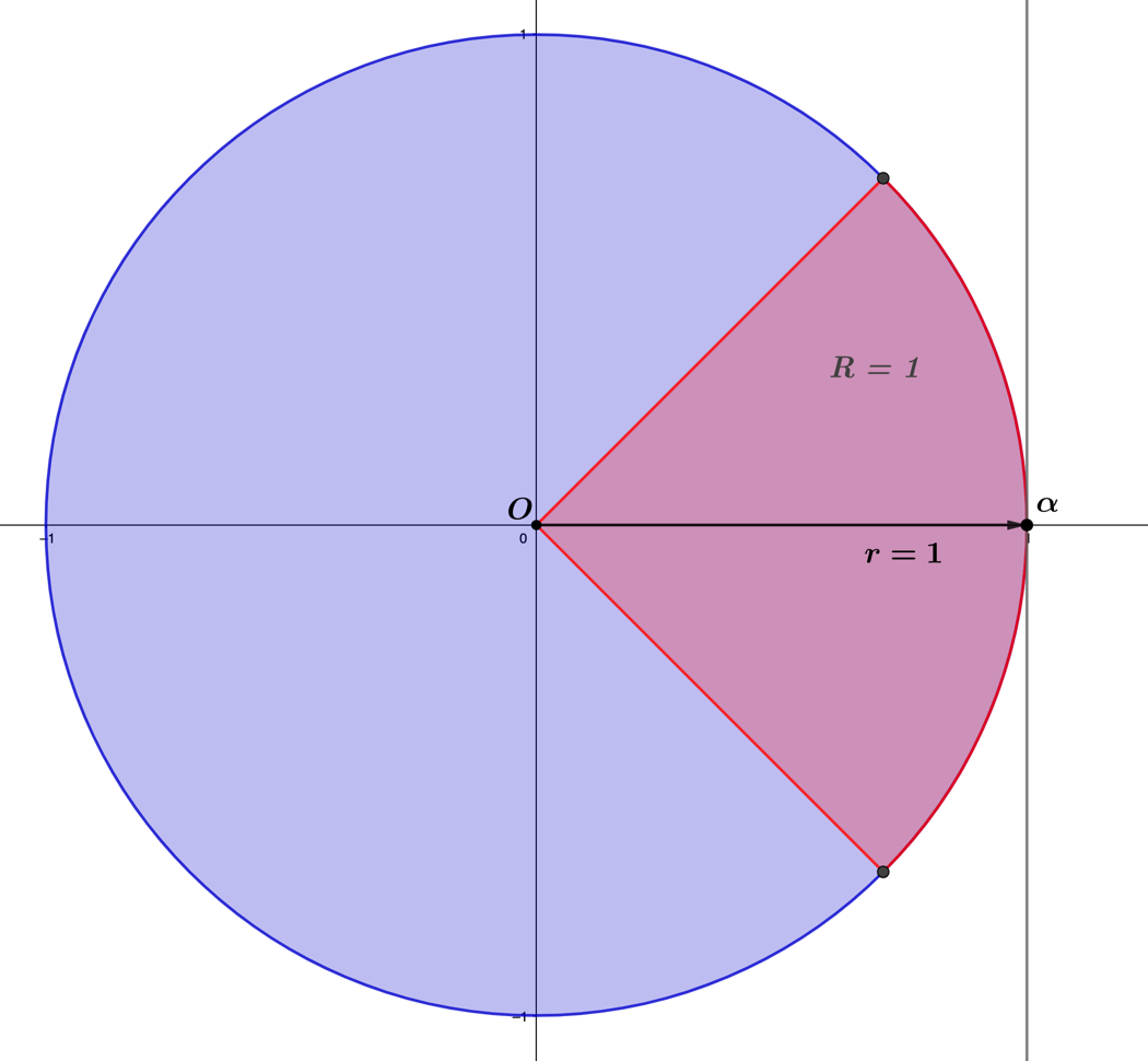
The radius of curvature for the unit circle is seen in Figure 1.3.11, for the circular arc of radius $R =$ 1, spanning from $e^{\left( \frac{- i\pi}{4} \right)}$ to $e^{\left( \frac{i\pi}{4} \right)}$ , reflecting the radius of curvature for the circle at the point $\alpha$ tangent to the boundary of the unit circle. As the radius of the circle being considered becomes very large in magnitude, the circular arc for the radius of curvature becomes much flatter. For a circular arc of defined length, we can determine the symmetric bounds of a counterpart circular arc of the same arc length by using the following equivalence

\begin{array}{r} \int_{a_{1}}^{b_{1}}{r_{1}\ dt} = \int_{a_{2}}^{b_{2}}{r_{2}\ dt}, \end{array}

(1.3.78)

for which, $r_{1},r_{2}$ are the known radii of the circular arcs, and the integration bounds are known for the defined circular arc. Using our unit circle example for the bounds $a_{1} = - \frac{\pi}{4},\ b_{1} = \frac{\pi}{4}$ , we compare this to a circular arc of radius $r = 25$ , to find the symmetric bounds equal

\int_{- \frac{\pi}{4}}^{\frac{\pi}{4}}{\ 1\ dt} = \int_{a_{2}}^{b_{2}}{25\ dt} \rightarrow \frac{\pi}{2} = \left. \ 25t \right|_{a_{2}}^{b_{2}}

\begin{array}{r} \rightarrow \frac{\pi}{2} = 25\left( b_{2} - a_{2} \right) \rightarrow \frac{\pi}{50} = \left( b_{2} - a_{2} \right), \end{array}

(1.3.79)

where this result represents the known bound multiplied by the inverse radius $\frac{\pi}{2r}.$

Figure 1.3.11 -The radius of curvature $R$ at the point $\alpha$ on the unit circle, with a

vertical line at $x = 1$ , representing the zero curvature of the line.

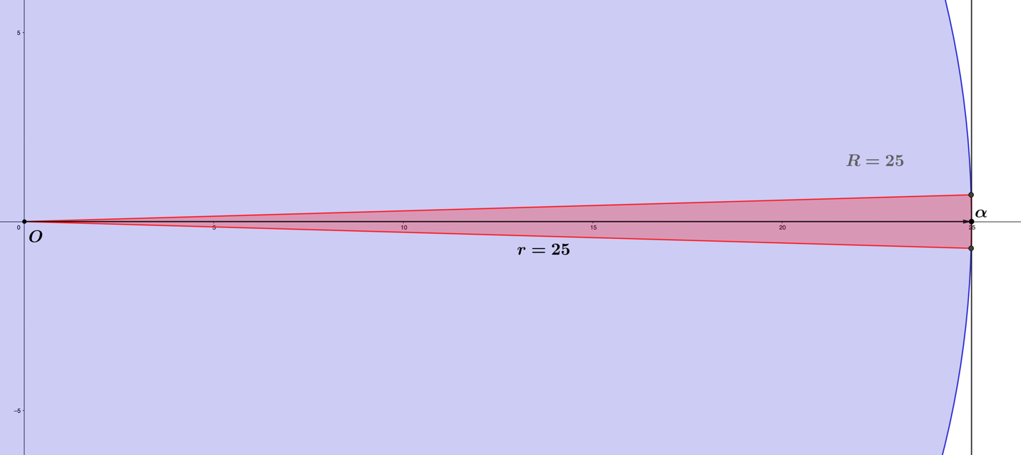
By assuming symmetric bounds about the positive real-axis of the circle for $a_{2}$ and $b_{2}$ , we define the values $a_{2} = - \frac{\pi}{100},b_{2} = \frac{\pi}{100},$ and plot the circle of radius $r = 25$ using a circular arc length equal to $\frac{\pi}{2}$ , which is equal to the previous unit circle example (Figure 1.3.12). Since the factor $1/r$ represents the curvature of the circle, we can also express a generalization of the integral equivalence in terms of $\kappa$ , as

\begin{array}{r} \int_{- a_{1}}^{b_{1}}{1\ dt} = \int_{- \frac{a_{1}}{r}}^{\frac{b_{1}}{r}}{\ \frac{1}{\kappa}\ dt}. \end{array}

(1.3.80)

Figure 1.3.12 -The circular arc for the radius of curvature $R$ at the point $\alpha$ on the

circle $x^{2} + y^{2} = 25^{2}$ , tending to the flatness of the line defined at $x = 25.$

Since $\kappa$ is a constant, we can factor it out of the integral, then solve for $\kappa$

\begin{array}{r} \int_{- a_{1}}^{b_{1}}{1\ dt} = \int_{- \frac{a_{1}}{r}}^{\frac{b_{1}}{r}}{\frac{1}{\kappa}\ dt} \rightarrow \int_{- a_{1}}^{b_{1}}{1\ dt} = \frac{1}{\kappa}\int_{- \frac{a_{1}}{r}}^{\frac{b_{1}}{r}}{1\ dt} \rightarrow \kappa = \frac{\int_{- \frac{a_{1}}{r}}^{\frac{b_{1}}{r}}{1\ dt}}{\int_{- a_{1}}^{b_{1}}{1\ dt}}, \end{array}

(1.3.81)

finding that the curvature of a circle can be expressed as the ratio of the arclength integrals on the unit circle. Solving these arclength integrals, we find

\begin{array}{r} \kappa = \frac{\int_{- \frac{a_{1}}{r}}^{\frac{b_{1}}{r}}{1\ dt}}{\int_{- a_{1}}^{b_{1}}{1\ dt}} = \frac{\left. \ t \right|_{- \frac{a_{1}}{r}}^{\frac{b_{1}}{r}}}{\left. \ t \right|_{- a_{1}}^{b_{1}}} = \frac{\left( \frac{b_{1}}{r} + \frac{a_{1}}{r} \right)}{\left( b_{1} + a_{1} \right)} = \frac{1}{r}, \end{array}

(1.3.82)

where the curvature result is as expected for the circle. Therefore, the product of the circle's curvature with its radius is equal to the identity

\begin{array}{r} \kappa r = \epsilon. \end{array}

(1.3.83)

Thinking about circular curvature as the ratio between the equal arclengths has important applications. In the next section, we will expand on this process to find the wave-like means by which we can represent circular curvature.

Text size

Light or dark

Look