1.3.5 Circular Curvature and the Wave Equation

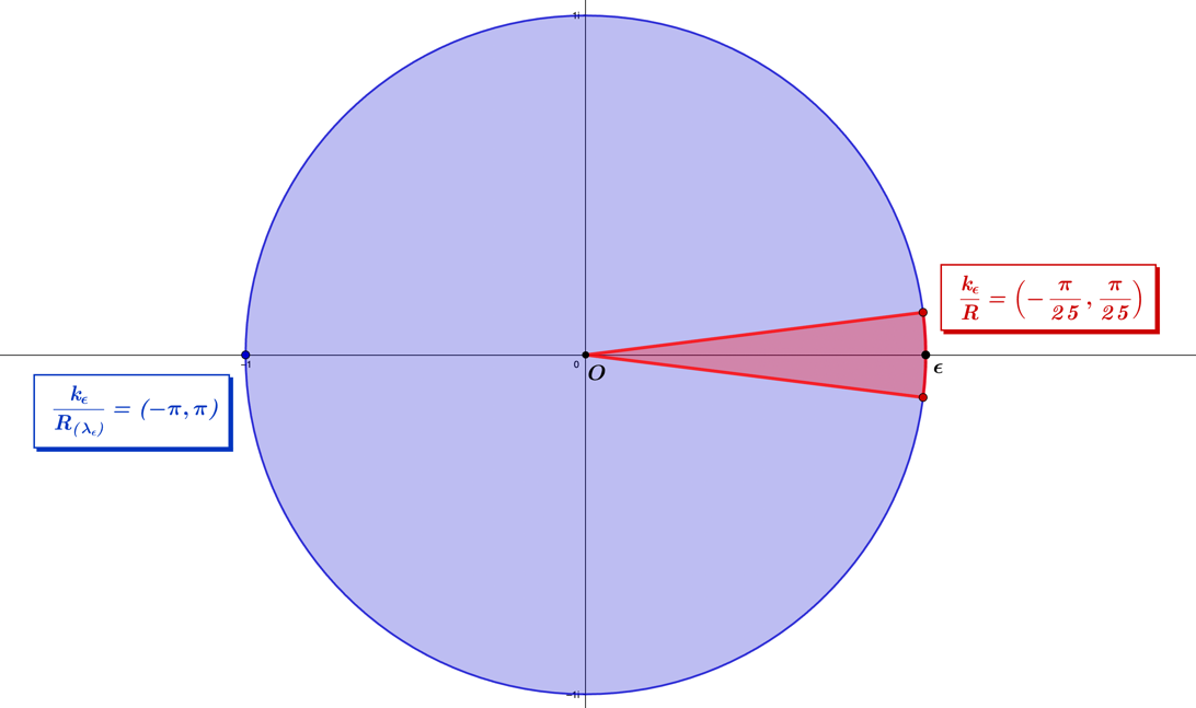
In the last sec­tion, we used images that showed cir­cu­lar arcs of the unit circle and com­pared them to arcs on a much larger circle of radius $r = 25.$In this sec­tion, we again apply cir­cu­lar arcs and the radius of cur­va­ture with a stan­dard­ized ar­clength for the unit circle. By doing so, we find ex­pres­sions in the form of dif­fer­en­tial equa­tions that enable us to ex­press cur­va­ture in terms of the wave equa­tion. From the ex­am­ple cir­cles in the last sec­tion, we ex­press the equiv­a­lence from Eq. 1.3.78 in the fol­low­ing form

Above, $R_{\epsilon}$ rep­re­sents the uni­tary spa­tial radius of the unit circle, $R$ is the radius of an­oth­er circle of pre­sum­ably dif­fer­ing radius, and equal­ly split wave num­bers in ra­di­ans rep­re­sent the bounds of in­te­gra­tion for both. Solv­ing this ex­pres­sion for $\frac{R_{\epsilon}}{R}$ re­sults in the ratio ex­pres­sion of radii to that of unit circle ar­clength in­te­grals

This ex­pres­sion is like that found in the last sec­tion for cir­cu­lar cur­va­ture, and this result can be gen­er­al­ized to any two cir­cles of dif­fer­ent radii with equal ar­clengths, as

for which, $R_{1} < R_{2}.$This can be stated in cur­va­ture no­ta­tion,

and eval­u­at­ing the in­te­grals, we find a form like the case of the unit circle,

im­ply­ing the ratio of the cur­va­tures of two cir­cles can be stated by a wave number de­pen­den­cy. By set­ting $R_{1} = R_{\epsilon}$, and $R_{2} = R$, the result above sim­pli­fies to the form

which rep­re­sents the $\frac{dx}{ds}$ por­tion of the cur­va­ture ex­pres­sion

Since we are con­sid­er­ing cir­cles with equal ar­clengths, this yields the iden­ti­ty equiv­a­lence

Noting the fol­low­ing iden­ti­ties for the wavenum­ber $k$, and the an­gu­lar fre­quen­cy $\omega$,

for $\lambda$, the wave­length and $T$, the period. There­fore, we can define the stan­dard wave number $k_{\epsilon}$, and an­gu­lar fre­quen­cy $\omega_{\epsilon}$, for the unit circle, as the fol­low­ing

The wave number is de­fined in ra­di­ans per unit dis­tance in space, while the an­gu­lar fre­quen­cy is de­fined in ra­di­ans per unit dis­tance in time. This means the uni­tary values for $\lambda$,$\ T$ in the stan­dard­iza­tions differ from each other, and to ac­count for this, $k_{\epsilon}$, $\omega_{\epsilon}$ can be rewrit­ten, as

where $T_{\epsilon}$ rep­re­sents the unit period dis­tance in time and $\lambda_{\epsilon}$ rep­re­sents the unit wave­length dis­tance in space. With these stan­dards, we can ex­press the unit an­gu­lar fre­quen­cy as the fol­low­ing ar­clength in­te­gral, for $R_{\left( T_{\epsilon} \right)} = \frac{1}{T_{\epsilon}}$,

and the unit wave number, for $R_{\left( \lambda_{\epsilon} \right)} = \ \frac{1}{\lambda_{\epsilon}}$, as

where the radial unit dis­tance in time $R_{\left( T_{\epsilon} \right)}$, and the radial unit dis­tance in space $R_{\left( \lambda_{\epsilon} \right)}$, are dis­cerned. The sim­i­lar­i­ty be­tween the stan­dard­iza­tions and the re­duced Planck's con­stant $\hslash$ should be noted

in which, $h$ rep­re­sents Planck's con­stant. The ar­clength equal­i­ty in the pre­vi­ous sec­tion can now be eval­u­at­ed using the wave number stan­dard­iza­tion $k_{\epsilon} = \frac{2\pi}{\lambda_{\epsilon}}$, as

and the figure below shows a plot of the com­par­a­tive cir­cu­lar arcs for each con­ver­gence radius.

fre­quen­cy of the unit circle in blue, $\frac{k_{\epsilon}}{R\left( \lambda_{\epsilon} \right)} = ( - \pi,\pi)$, and the circle of radius, $R = 25$, in red,$\frac{k_{\epsilon}}{R} = \left( - \frac{\pi}{25},\frac{\pi}{25} \right).$

Space cur­va­ture for the circle is the typ­i­cal math­e­mat­i­cal treat­ment we en­counter, and it can be pa­ram­e­trized into the spa­tial form

The ar­clength $A\left( \gamma(s) \right)$, will have the in­te­gral rep­re­sen­ta­tion,

which eval­u­ates to the squared wave number

The ar­clength with unit spa­tial domain bounds of in­te­gra­tion is ex­pressed, as

and this in­te­gral eval­u­ates to

where the prod­uct of the unit wavenum­ber $2\pi k$, and the wavenum­ber rep­re­sen­ta­tion of the non-uni­tary radius circle are con­sid­ered

Cir­cu­lar cur­va­ture can be ex­pressed as a ratio of the ar­clengths $A\left( \gamma(s) \right)$/$A\left( \gamma_{\epsilon}(s) \right)$, equal­ing the in­verse wave­length seen as fol­lows

Since $\lambda$ is the spa­tial ex­ten­sion rep­re­sent­ing the circle's radius, the cur­va­ture is equal to the in­verse of the radius $R_{s}$ of the spa­tial circle

Simply put, space cur­va­ture is the ratio of the said wavenum­ber $k$, with that of the unit circle's $k_{\epsilon} = \frac{2\pi}{1}$

Cur­va­ture also exists in the fre­quen­cy domain in the form of time cur­va­ture, seen by using the fol­low­ing time-based pa­ram­e­triza­tion

The ar­clength in the fre­quen­cy domain has the in­te­gral rep­re­sen­ta­tion

and like its spa­tial coun­ter­part, will eval­u­ate to the squared an­gu­lar fre­quen­cy,

The ar­clength with unit fre­quen­cy domain bounds of in­te­gra­tion, takes the fol­low­ing in­te­gral form,

which eval­u­ates to

where $2\pi\omega$ can also be con­sid­ered as a prod­uct of $\omega_{\epsilon}$ and $\omega$,

Like the spa­tial domain, cir­cu­lar cur­va­ture in the fre­quen­cy domain is a ratio of arc lengths $A\left( \gamma(t) \right)$/$A\left( \gamma_{\epsilon}(t) \right)$, and equals the in­verse period

Since $T$ is the time ex­ten­sion that rep­re­sents the radius of the circle, the cur­va­ture is also equal to the in­verse of the radius $R_{t}$ of the circle

and in the fre­quen­cy domain, the cur­va­ture is the ratio of the said an­gu­lar fre­quen­cy, $\omega$, with that of the unit circle's, $\omega_{\epsilon} = \frac{2\pi}{1}$

We apply our ar­clength for­mu­las to derive the fol­low­ing in­fin­i­tes­i­mals, where the spa­tial in­fin­i­tes­i­mal is the wavenum­ber

and the tem­po­ral in­fin­i­tes­i­mal is the an­gu­lar fre­quen­cy

As­sum­ing we are deal­ing with elec­tro­mag­net­ic waves, the prod­uct of the in­verse space cur­va­ture with the time cur­va­ture, equals the speed of light

Putting cur­va­ture in the per­spec­tive of both the fre­quen­cy and spa­tial do­mains en­ables us to derive the wave equa­tion from their rep­re­sen­ta­tions. To start, we put the spa­tial and tem­po­ral domain pa­ram­e­triza­tions in their com­plex forms as

and their prod­uct is the plane wave equa­tion

Given that $\gamma(t,x)$ is the prod­uct of two func­tions $\gamma(x)\gamma(t)$, it will form a sep­a­ra­ble par­tial dif­fer­en­tial equa­tion. Using $\gamma(t,x)$, we eval­u­ate the second-order time de­riv­a­tive

and the second-order spa­tial de­riv­a­tive

Next, we con­sid­er the fol­low­ing dif­fer­en­tial equa­tion

where $\alpha$ is the value that en­ables the equa­tion to be true. We sub­sti­tute the second-order de­riv­a­tive re­sults into the dif­fer­en­tial equa­tion and solve for $\alpha$, as fol­lows

and by the iden­ti­ty

this im­plies that $\alpha$, as­sum­ing elec­tro­mag­net­ic forms, equals

lead­ing to the wave equa­tion for­mal­ism

Using our in­verse cir­cu­lar radius re­sults for the time and spa­tial do­mains cur­va­tures,

we con­sid­er $\alpha$

and al­ge­braical­ly modify it, as fol­lows

We sub­sti­tute this result back into our wave equa­tion

and then re­arrange it to

Im­plic­it in this form is some­thing very re­veal­ing con­cern­ing, $\frac{\lambda^{2}}{T^{2}} = c^{2}$; since $\lambda$ is the dis­tance in space, and $T$ is the dis­tance in time, which im­plies the speed of light is com­posed of space and time pro­por­tions that are equal in mag­ni­tude. For cir­cu­lar cur­va­ture, the dis­tance in space and time re­quired to have uni­tary cur­va­ture are found to be the fol­low­ing

where $R_{s}$ rep­re­sents the radial dis­tance in space and $R_{t}$ rep­re­sents the radial dis­tance in time. This re­sults in the equiv­a­lence

and given that $\lambda_{\epsilon}$ is the unit dis­tance of space and $T_{\epsilon}$ us the unit dis­tance of time*,* the time and space units of dis­tance cancel in the ratio, re­sult­ing in the iden­ti­ty

Using our unit circle ex­am­ple with in­te­gra­tion bounds $a_{1} = - \frac{\pi}{4},\ b_{1} = \frac{\pi}{4}$, we com­pare this to a cir­cu­lar arc of radius $r = 25$, to find the sym­met­ric bounds equal

This result rep­re­sents the known bound mul­ti­plied by the in­verse radius $\frac{\pi}{2r}$, which can also be ex­pressed in cur­va­ture no­ta­tion, as

This im­plies for cir­cu­lar cur­va­ture ap­pli­ca­tions, that

which is con­sis­tent with what was found in the case of the first-order de­riv­a­tive

where the mag­ni­tude of a change in the dis­tance in space is equal to the mag­ni­tude of a change in the dis­tance in time

Once again, using $\gamma(t,x)$, we con­sid­er the first-order time de­riv­a­tive

and the first-order spa­tial de­riv­a­tive

to con­sid­er the first-order dif­fer­en­tial equa­tion

by solv­ing for $\alpha$

By putting the vari­able $\alpha$ into the con­text of cur­va­ture, we can ex­press the dif­fer­en­tial equa­tion in the fol­low­ing form

and with re­arrange­ments, this leads to the fol­low­ing space and time cur­va­ture so­lu­tions

The light speed ex­pres­sion

then leads to the fol­low­ing space and time cur­va­ture ex­pres­sions

which shows cur­va­ture and light are in­ter­twined.