The last section saw how the infinite integration of a projected form of oriented vectors could yield a similar result to exponentiation. The ability to integrate these projected forms implies the existence of differential forms. This chapter will discuss tangent spaces and tangent vectors of Lie groups and their relationship to the Lie algebras of that group. Lie groups will typically be non-Euclidean, but remarkably, it is possible to reveal the Lie algebra underlying the group through its tangent space, which is a distinctly Euclidean concept. For a smooth path through the Lie group, where smooth means that a derivative exists, the tangent space is captured through the tangent vectors passing through the identity.
Before getting into the details surrounding tangent spaces, we must consider matrix derivatives. Our first step is to update our element notation to help avoid any confusion as we proceed. For each of the D 3 ℝ , D 3 ℂ , D 3 𝕔 D_{3\mathbb{R}},\ D_{3\mathbb{C}},\ D_{3\mathbb{c}} X j , Y j X_{j},Y_{j} X j , Y j ∈ A X_{j},Y_{j} \in A
D 3 ℝ : A ℝ = { X j ℝ , Y k ℝ } , D 3 ℂ : A ℂ = { X j , k ℂ , Y j , k ℂ } , D 3 𝕔 : A 𝕔 = { X j , k 𝕔 , Y j , k 𝕔 } , \begin{array}{r}
D_{3\mathbb{R}}:\ A_{\mathbb{R}} = \left\{ X_{j}^{\mathbb{R}},Y_{k}^{\mathbb{R}} \right\},\ \ D_{3\mathbb{C}}\ :A_{\mathbb{C}} = \left\{ X_{j,k}^{\mathbb{C}},Y_{j,k}^{\mathbb{C}} \right\},\ \ D_{3\mathbb{c}}\ :A_{\mathbb{c}} = \left\{ X_{j,k}^{\mathbb{c}},Y_{j,k}^{\mathbb{c}} \right\},
\end{array} (1.2.1) where we will refer to the S 3 ℝ / D 3 ℝ S_{3\mathbb{R}}/D_{3\mathbb{R}} D 3 ℝ D_{3\mathbb{R}} 𝕔 \mathbb{c} ( a + i b ) = r e i x j {(a + ib) = re}^{ix_{j}} r , x j ∈ ℝ {r,x}_{j}\in \mathbb{R} D 3 ℂ D_{3\mathbb{C}} D 3 𝕔 {\ D}_{3\mathbb{c}} A A
A = { A ℝ , A ℂ , A 𝕔 } , \begin{array}{r}
A = \left\{ A_{\mathbb{R}},A_{\mathbb{C}},A_{\mathbb{c}} \right\},
\end{array} (1.2.2) the exponential mappings of the X j X_{j} Y j Y_{j} ∈ A \in A G ( x j X j ) , G ( y j Y j ) G\left( {x_{j}X}_{j} \right),G\left( y_{j}Y_{j} \right)
e t A : → G ( x j X j ) , G ( y j Y j ) = e x j X j , e y j Y j , \begin{array}{r}
e^{tA}: \rightarrow G\left( x_{j}X_{j} \right),G\left( y_{j}Y_{j} \right) = e^{x_{j}X_{j}},e^{y_{j}Y_{j}},
\end{array} (1.2.3) for variables x j , y j ∈ ℝ . x_{j},y_{j}\in \mathbb{R}. G ( x j X j ) G\left( {x_{j}X}_{j} \right) G ( y j Y j ) G\left( y_{j}Y_{j} \right)
d d x j G ( x j X j ) = G ′ ( x j X j ) , d d y j G ( y j Y j ) = G ′ ( y j Y j ) , \begin{array}{r}
\frac{d}{dx_{j}}G\left( {x_{j}X}_{j} \right) = G^{'}\left( {x_{j}X}_{j} \right),\ \ \frac{d}{dy_{j}}G\left( y_{j}Y_{j} \right) = G^{'}\left( y_{j}Y_{j} \right),
\end{array} (1.2.4) which have derivative algebras defined as
( x j X j ) ′ = ln ( G ′ ( x j X j ) ) , ( y j Y j ) ′ = ln ( G ′ ( y j Y j ) ) , \begin{array}{r}
\left( {x_{j}X}_{j} \right)^{'} = \ln\left( G^{'}\left( {x_{j}X}_{j} \right) \right),\ \left( y_{j}Y_{j} \right)^{'} = \ln{\left( G^{'}\left( y_{j}Y_{j} \right) \right),}
\end{array} (1.2.5) and since the matrix logarithm and exponential functions are inversely related, we have the identities
e ( x j X j ) ′ = G ′ ( x j X j ) , e ( y j Y j ) ′ = G ′ ( y j Y j ) . \begin{array}{r}
e^{\left( {x_{j}X}_{j} \right)^{'}} = G^{'}\left( {x_{j}X}_{j} \right),\ \ e^{\left( y_{j}Y_{j} \right)^{'}} = G^{'}\left( y_{j}Y_{j} \right).
\end{array} (1.2.6) In matrix calculus, it should be noted that there are different approaches to the differentiation of a matrix group. This chapter will use the matrix-by-scalar derivative technique to yield the tangent matrix . As the name implies, for an m × n m \times n G G
d G d t = ( ∂ g 1,1 ∂ t ∂ g 1,2 ∂ t … ∂ g 1 , n ∂ t ∂ g 2,1 ∂ t ∂ g 2,2 ∂ t … ∂ g 2 , n ∂ t ⋮ ⋮ ⋱ ⋮ ∂ g m , 1 ∂ t ∂ g m , 2 ∂ t … ∂ g m , n ∂ t ) . \begin{array}{r}
\frac{dG}{dt} = \begin{pmatrix}
\frac{\partial g_{1,1}}{\partial t} & \frac{\partial g_{1,2}}{\partial t} & \ldots & \frac{\partial g_{1,n}}{\partial t} \\
\frac{\partial g_{2,1}}{\partial t} & \frac{\partial g_{2,2}}{\partial t} & \ldots & \frac{\partial g_{2,n}}{\partial t} \\
\vdots & \vdots & \ddots & \vdots \\
\frac{\partial g_{m,1}}{\partial t} & \frac{\partial g_{m,2}}{\partial t} & \ldots & \frac{\partial g_{m,n}}{\partial t}
\end{pmatrix}.
\end{array} (1.2.7) We return to the infinite integration functions to consider their differential forms.
Definitions (1.2.8) For the vector 𝒸 x j \mathcal{c}x_{j} , where x j x_{j} is a unit basis vector of some n n -dimensional vector space, and 𝒸 \mathcal{c} is a scalar constant , , the derivative of the infinite integration functions f ℝ − ∞ ( 𝒸 x j ) a n d f ℂ − ∞ ( 𝒸 i x j ) f_{\mathbb{R}}^{- \infty}\left( \mathcal{c}x_{j} \right)\ and\ f_{\mathbb{C}}^{- \infty}\left( \mathcal{c}ix_{j} \right) starting at the zero point, for 𝒸 x j ∈ ℝ , 𝒸 i x j ∈ ℂ \mathcal{c}x_{j}\in \mathbb{R},\ \mathcal{c}ix_{j}\in \mathbb{C} , are defined as
D 1 [ f ℝ − ∞ ( 𝒸 x j ) ] = d d x j [ f ℝ − ∞ ( 𝒸 x j ) ] { ∀ 𝒸 ∈ ℝ , ∀ x j ∈ ℝ n } = d d x j [ 𝒸 e x j ] , \begin{array}{r}
D^{1}\left\lbrack f_{\mathbb{R}}^{- \infty}\left( \mathcal{c}x_{j} \right) \right\rbrack = \frac{d}{dx_{j}}\left\lbrack f_{\mathbb{R}}^{- \infty}\left( \mathcal{c}x_{j} \right) \right\rbrack\ \left\{ \forall\ \mathcal{c}\in \mathbb{R}\ ,\forall\ x_{j} \in \mathbb{R}^{n}\ \right\} = \frac{d}{dx_{j}}\left\lbrack {\mathcal{c}e}^{x_{j}} \right\rbrack,
\end{array} D 1 [ f ℂ − ∞ ( 𝒸 i x j ) ] = d d x j [ f ℂ − ∞ ( 𝒸 i x j ) ] { ∀ 𝒸 ∈ ℝ , ∀ x j ∈ ℝ n } = d d x j [ 𝒸 e i x j ] . D^{1}\left\lbrack f_{\mathbb{C}}^{- \infty}\left( \mathcal{c}ix_{j} \right) \right\rbrack = \frac{d}{dx_{j}}\left\lbrack f_{\mathbb{C}}^{- \infty}\left( \mathcal{c}ix_{j} \right) \right\rbrack\ \left\{ \forall\ \mathcal{c}\in \mathbb{R}\ ,\forall\ x_{j} \in \mathbb{R}^{n}\ \right\} = \frac{d}{dx_{j}}\left\lbrack {\mathcal{c}e}^{ix_{j}} \right\rbrack. Theorem (1.2.9) –Taking a unit basis vector x j x_{j} as a fixed form element, the functions D k [ f ℝ − ∞ ( 𝒸 x j ) ] , D k [ f ℂ − ∞ ( 𝒸 i x j ) ] D^{k}\left\lbrack f_{\mathbb{R}}^{- \infty}\left( \mathcal{c}x_{j} \right) \right\rbrack,D^{k}\left\lbrack f_{\mathbb{C}}^{- \infty}\left( \mathcal{c}ix_{j} \right) \right\rbrack are equal to the first derivatives of the exponential mapping e x p : 𝔤 → G ∈ ℝ , ℂ exp:\mathfrak{g} \rightarrow G\in \mathbb{R},\mathbb{C} onto a continuous manifold ∀ 𝔤 = x j \forall\ \mathfrak{g} =x_{j} .
Proof -
∀ 𝔤 = { x j } , ( e x p : 𝔤 ) ′ → G ′ = ( ∑ n = 0 ∞ ( x j ) n n ! ) ′ , \begin{array}{r}
\forall\ \mathfrak{g} ={\{ x}_{j}\},\ \ \ (exp:\mathfrak{g})' \rightarrow G' = \left( \sum_{n = 0}^{\infty}\frac{\left( x_{j} \right)^{n}}{n!} \right)^{'},
\end{array} D 1 [ f ℝ − ∞ ( 𝒸 x j ) ] = ( … + x j 5 120 + x j 4 24 + x j 3 6 + x j 2 2 + x j + 1 ) ′ = ( ∑ n = 0 ∞ ( x j ) n n ! ) ′ = ( e x p : 𝔤 ) ′ → G ′ ∀ 𝔤 = { x j } , \begin{array}{r}
D^{1}\left\lbrack f_{\mathbb{R}}^{- \infty}\left( \mathcal{c}x_{j} \right) \right\rbrack = \left( \ldots + \frac{x_{j}^{5}}{120} + \frac{x_{j}^{4}}{24} + \frac{x_{j}^{3}}{6} + \frac{x_{j}^{2}}{2} + x_{j} + 1 \right)^{'} = \left( \sum_{n = 0}^{\infty}\frac{\left( x_{j} \right)^{n}}{n!} \right)^{'} = \ (exp:\mathfrak{g})' \rightarrow G'\ \forall\ \mathfrak{g} ={\{ x}_{j}\},
\end{array} as
D 1 [ f ℝ − ∞ ( 𝒸 x j ) ] = ( … + x j 5 120 + x j 4 24 + x j 3 6 + x j 2 2 + x j + 1 ) ′ = ( … + x j 4 24 + x j 3 6 + x j 2 2 + x j 1 1 + x j 0 ) = G ′ , \begin{array}{r}
D^{1}\left\lbrack f_{\mathbb{R}}^{- \infty}\left( \mathcal{c}x_{j} \right) \right\rbrack = \left( \ldots + \frac{x_{j}^{5}}{120} + \frac{x_{j}^{4}}{24} + \frac{x_{j}^{3}}{6} + \frac{x_{j}^{2}}{2} + x_{j} + 1 \right)^{'} = {\left( \ldots + \frac{x_{j}^{4}}{24} + \frac{x_{j}^{3}}{6} + \frac{x_{j}^{2}}{2} + \frac{x_{j}^{1}}{1} + x_{j}^{0} \right) = G}^{'},
\end{array} and for D 1 [ f ℂ − ∞ ( 𝒸 i x j ) ] D^{1}\left\lbrack f_{\mathbb{C}}^{- \infty}\left( \mathcal{c}ix_{j} \right) \right\rbrack
D 1 [ f ℂ − ∞ ( 𝒸 i x j ) ] = ( … + ( i x j ) 5 120 + ( i x j ) 4 24 + ( i x j ) 3 6 + ( i x j ) 2 2 + i x j + 1 ) ′ = ( ∑ n = 0 ∞ ( i x j ) n n ! ) ′ = e x p : 𝔤 → G ∀ 𝔤 = { i x j } , \begin{array}{r}
D^{1}\left\lbrack f_{\mathbb{C}}^{- \infty}\left( \mathcal{c}ix_{j} \right) \right\rbrack = \left( \ldots + \frac{\left( ix_{j} \right)^{5}}{120} + \frac{\left( ix_{j} \right)^{4}}{24} + \frac{\left( ix_{j} \right)^{3}}{6} + \frac{\left( ix_{j} \right)^{2}}{2} + ix_{j} + 1\ \right)^{'} = \left( \sum_{n = 0}^{\infty}\frac{\left( {ix}_{j} \right)^{n}}{n!} \right)^{'} = exp:\mathfrak{g} \rightarrow G\ \forall\ \mathfrak{g} ={\{ ix}_{j}\},
\end{array} as
D 1 [ f ℂ − ∞ ( 𝒸 i x j ) ] = ( … + ( i x j ) 5 120 + ( i x j ) 4 24 + ( i x j ) 3 6 + ( i x j ) 2 2 + i x j + 1 ) ′ = … + ( i x j ) 4 24 + ( i x j ) 3 6 + ( i x j ) 2 2 + ( i x j ) 1 1 + i x j 0 . \begin{array}{r}
D^{1}\left\lbrack f_{\mathbb{C}}^{- \infty}\left( \mathcal{c}ix_{j} \right) \right\rbrack = \left( \ldots + \frac{\left( ix_{j} \right)^{5}}{120} + \frac{\left( ix_{j} \right)^{4}}{24} + \frac{\left( ix_{j} \right)^{3}}{6} + \frac{\left( ix_{j} \right)^{2}}{2} + ix_{j} + 1\ \right)^{'} = \ldots + \frac{\left( ix_{j} \right)^{4}}{24} + \frac{\left( ix_{j} \right)^{3}}{6} + \frac{\left( ix_{j} \right)^{2}}{2} + \frac{\left( ix_{j} \right)^{1}}{1} + ix_{j}^{0}.
\end{array} □ \square We apply this derivative approach for our exponentiated permutations in the examples above to find D 1 [ 𝒸 e X 3 ] D^{1}\left\lbrack \mathcal{c}e^{X_{3}} \right\rbrack
D 1 [ 𝒸 e X 3 ] = d d x 3 𝒸 ( 1 − x 3 2 2 ! + x 3 4 4 ! + … i x 3 − i x 3 3 3 ! + i x 3 5 5 ! + … 0 i x 3 − i x 3 3 3 ! + i x 3 5 5 ! + … 1 − x 3 2 2 ! + x 3 4 4 ! + … 0 0 0 1 + i x 3 − x 3 2 2 ! − i x 3 3 3 ! + x 3 4 4 ! + i x 3 5 5 ! + … ) → D^{1}\left\lbrack \mathcal{c}e^{X_{3}} \right\rbrack = \frac{d}{dx_{3}}\mathcal{c}\begin{pmatrix}
1 - \frac{x_{3}^{2}}{2!} + \frac{x_{3}^{4}}{4!} + \ldots & ix_{3} - \frac{{ix}_{3}^{3}}{3!} + \frac{ix_{3}^{5}}{5!} + \ldots & 0 \\
ix_{3} - \frac{{ix}_{3}^{3}}{3!} + \frac{ix_{3}^{5}}{5!} + \ldots & 1 - \frac{x_{3}^{2}}{2!} + \frac{x_{3}^{4}}{4!} + \ldots & 0 \\
0 & 0 & 1 + ix_{3} - \frac{x_{3}^{2}}{2!} - \frac{{ix}_{3}^{3}}{3!} + \frac{x_{3}^{4}}{4!} + \frac{ix_{3}^{5}}{5!} + \ldots
\end{pmatrix} \rightarrow D 1 [ 𝒸 e X 3 ] = 𝒸 ( − x 3 + x 3 3 3 ! − x 3 5 5 ! + … i − i x 3 2 2 ! + i x 3 4 4 ! + … 0 i − i x 3 2 2 ! + i x 3 4 4 ! + … − x 3 + x 3 3 3 ! − x 3 5 5 ! + … 0 0 0 i − x 3 − i x 3 2 2 ! + x 3 3 3 ! + i x 3 4 4 ! − x 3 5 5 ! + … ) D^{1}\left\lbrack \mathcal{c}e^{X_{3}} \right\rbrack= \mathcal{c}\begin{pmatrix}
- x_{3} + \frac{x_{3}^{3}}{3!} - \frac{x_{3}^{5}}{5!} + \ldots & i - \frac{{ix}_{3}^{2}}{2!} + \frac{ix_{3}^{4}}{4!} + \ldots & 0 \\
i - \frac{{ix}_{3}^{2}}{2!} + \frac{ix_{3}^{4}}{4!} + \ldots & - x_{3} + \frac{x_{3}^{3}}{3!} - \frac{x_{3}^{5}}{5!} + \ldots & 0 \\
0 & 0 & i - x_{3} - \frac{{ix}_{3}^{2}}{2!} + \frac{x_{3}^{3}}{3!} + \frac{ix_{3}^{4}}{4!} - \frac{x_{3}^{5}}{5!} + \ldots
\end{pmatrix} = c ( − sin ( x 3 ) i c o s ( x 3 ) 0 i c o s ( x 3 ) − sin ( x 3 ) 0 0 0 i e i x 3 ) , \begin{array}{r}
= c\begin{pmatrix}
{- \sin}\left( x_{3} \right) & icos\left( x_{3} \right) & 0 \\
icos\left( x_{3} \right) & {- \sin}\left( x_{3} \right) & 0 \\
0 & 0 & {ie}^{ix_{3}}
\end{pmatrix},
\end{array} (1.2.10) and next, D 1 [ 𝒸 e Y 2 ] D^{1}\left\lbrack \mathcal{c}e^{Y_{2}} \right\rbrack
D 1 [ 𝒸 e Y 2 ] = d d y 2 𝒸 ( 1 + y 2 3 3 ! + y 2 6 6 ! + … y 2 + y 2 4 4 ! + y 2 7 7 ! + … y 2 2 2 ! + y 2 5 5 ! + y 2 8 8 ! + … y 2 2 2 ! + y 2 5 5 ! + y 2 8 8 ! + … 1 + y 2 3 3 ! + y 2 6 6 ! + … y 2 + y 2 4 4 ! + y 2 7 7 ! + … y 2 + y 2 4 4 ! + y 2 7 7 ! + … y 2 2 2 ! + y 2 5 5 ! + y 2 8 8 ! + … 1 + y 2 3 3 ! + y 2 6 6 ! + … ) → D^{1}\left\lbrack \mathcal{c}e^{Y_{2}} \right\rbrack = \frac{d}{dy_{2}}\mathcal{c}\begin{pmatrix}
1 + \frac{y_{2}^{3}}{3!} + \frac{y_{2}^{6}}{6!} + \ldots & y_{2} + \frac{y_{2}^{4}}{4!} + \frac{y_{2}^{7}}{7!} + \ldots & \frac{y_{2}^{2}}{2!} + \frac{y_{2}^{5}}{5!} + \frac{y_{2}^{8}}{8!} + \ldots \\
\frac{y_{2}^{2}}{2!} + \frac{y_{2}^{5}}{5!} + \frac{y_{2}^{8}}{8!} + \ldots & 1 + \frac{y_{2}^{3}}{3!} + \frac{y_{2}^{6}}{6!} + \ldots & y_{2} + \frac{y_{2}^{4}}{4!} + \frac{y_{2}^{7}}{7!} + \ldots \\
y_{2} + \frac{y_{2}^{4}}{4!} + \frac{y_{2}^{7}}{7!} + \ldots & \frac{y_{2}^{2}}{2!} + \frac{y_{2}^{5}}{5!} + \frac{y_{2}^{8}}{8!} + \ldots & 1 + \frac{y_{2}^{3}}{3!} + \frac{y_{2}^{6}}{6!} + \ldots
\end{pmatrix} \rightarrow D 1 [ 𝒸 e Y 2 ] = 𝒸 ( y 2 2 2 ! + y 2 5 5 ! + y 2 8 8 ! + … 1 + y 2 3 3 ! + y 2 6 6 ! + … y 2 + y 2 4 4 ! + y 2 7 7 ! + … y 2 + y 2 4 4 ! + y 2 7 7 ! + … y 2 2 2 ! + y 2 5 5 ! + y 2 8 8 ! + … 1 + y 2 3 3 ! + y 2 6 6 ! + … 1 + y 2 3 3 ! + y 2 6 6 ! + … y 2 + y 2 4 4 ! + y 2 7 7 ! + … y 2 2 2 ! + y 2 5 5 ! + y 2 8 8 ! + … ) → D^{1}\left\lbrack \mathcal{c}e^{Y_{2}} \right\rbrack= \mathcal{c}\begin{pmatrix}
\frac{y_{2}^{2}}{2!} + \frac{y_{2}^{5}}{5!} + \frac{y_{2}^{8}}{8!} + \ldots & 1 + \frac{y_{2}^{3}}{3!} + \frac{y_{2}^{6}}{6!} + \ldots & y_{2} + \frac{y_{2}^{4}}{4!} + \frac{y_{2}^{7}}{7!} + \ldots \\
y_{2} + \frac{y_{2}^{4}}{4!} + \frac{y_{2}^{7}}{7!} + \ldots & \frac{y_{2}^{2}}{2!} + \frac{y_{2}^{5}}{5!} + \frac{y_{2}^{8}}{8!} + \ldots & 1 + \frac{y_{2}^{3}}{3!} + \frac{y_{2}^{6}}{6!} + \ldots \\
1 + \frac{y_{2}^{3}}{3!} + \frac{y_{2}^{6}}{6!} + \ldots & y_{2} + \frac{y_{2}^{4}}{4!} + \frac{y_{2}^{7}}{7!} + \ldots & \frac{y_{2}^{2}}{2!} + \frac{y_{2}^{5}}{5!} + \frac{y_{2}^{8}}{8!} + \ldots
\end{pmatrix} \rightarrow D 1 [ 𝒸 e Y 2 ] = 𝒸 ( e y 2 3 − 2 3 e − y 2 2 sin ( π 6 + 3 y 2 2 ) e y 2 3 + 2 3 e − y 2 2 cos ( 3 y 2 2 ) e y 2 3 − 2 3 e − y 2 2 sin ( π 6 − 3 y 2 2 ) e y 2 3 − 2 3 e − y 2 2 sin ( π 6 − 3 y 2 2 ) e y 2 3 − 2 3 e − y 2 2 sin ( π 6 + 3 y 2 2 ) e y 2 3 + 2 3 e − y 2 2 cos ( 3 y 2 2 ) e y 2 3 + 2 3 e − y 2 2 cos ( 3 y 2 2 ) e y 2 3 − 2 3 e − y 2 2 sin ( π 6 − 3 y 2 2 ) e y 2 3 − 2 3 e − y 2 2 sin ( π 6 + 3 y 2 2 ) ) . \begin{array}{r}
\ D^{1}\left\lbrack \mathcal{c}e^{Y_{2}} \right\rbrack= \mathcal{c}\begin{pmatrix}
\frac{e^{y_{2}}}{3} - \frac{2}{3}e^{- \frac{y_{2}}{2}}\sin\left( \frac{\pi}{6} + \frac{\sqrt{3}y_{2}}{2} \right) & \frac{e^{y_{2}}}{3} + \frac{2}{3}e^{- \frac{y_{2}}{2}}\cos\left( \frac{\sqrt{3}y_{2}}{2} \right) & \frac{e^{y_{2}}}{3} - \frac{2}{3}e^{- \frac{y_{2}}{2}}\sin\left( \frac{\pi}{6} - \frac{\sqrt{3}y_{2}}{2} \right) \\
\frac{e^{y_{2}}}{3} - \frac{2}{3}e^{- \frac{y_{2}}{2}}\sin\left( \frac{\pi}{6} - \frac{\sqrt{3}y_{2}}{2} \right) & \frac{e^{y_{2}}}{3} - \frac{2}{3}e^{- \frac{y_{2}}{2}}\sin\left( \frac{\pi}{6} + \frac{\sqrt{3}y_{2}}{2} \right) & \frac{e^{y_{2}}}{3} + \frac{2}{3}e^{- \frac{y_{2}}{2}}\cos\left( \frac{\sqrt{3}y_{2}}{2} \right) \\
\frac{e^{y_{2}}}{3} + \frac{2}{3}e^{- \frac{y_{2}}{2}}\cos\left( \frac{\sqrt{3}y_{2}}{2} \right) & \frac{e^{y_{2}}}{3} - \frac{2}{3}e^{- \frac{y_{2}}{2}}\sin\left( \frac{\pi}{6} - \frac{\sqrt{3}y_{2}}{2} \right) & \frac{e^{y_{2}}}{3} - \frac{2}{3}e^{- \frac{y_{2}}{2}}\sin\left( \frac{\pi}{6} + \frac{\sqrt{3}y_{2}}{2} \right)
\end{pmatrix}.
\end{array} (1.2.11) We can see that for D 1 [ 𝒸 e Y 2 ] D^{1}\left\lbrack \mathcal{c}e^{Y_{2}} \right\rbrack D 1 [ 𝒸 e Y 3 ] D^{1}\left\lbrack \mathcal{c}e^{Y_{3}} \right\rbrack U ( 3 ) U(3) D 1 [ 𝒸 e i X 3 ] = G ′ ( i X 3 ) D^{1}\left\lbrack \mathcal{c}e^{iX_{3}} \right\rbrack = G^{'}\left( iX_{3} \right) f ℂ ′ ( i X 3 ) f_{\mathbb{C}}'\left( iX_{3} \right) i π 4 \frac{i\pi}{4}
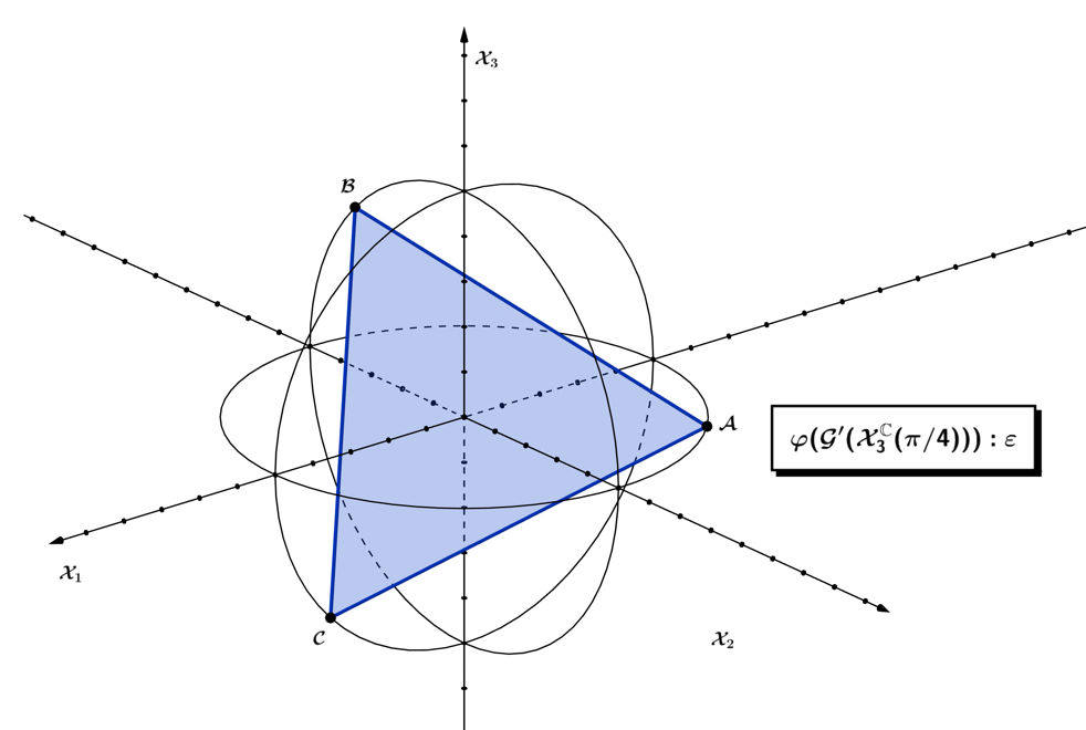
ϕ ( G ′ ( X 3 ℂ ( π 4 ) ) : ϵ ) = ( − s i n ( π 4 ) i c o s ( π 4 ) 0 i c o s ( π 4 ) − s i n ( π 4 ) 0 0 0 i e ( i π 4 ) ) ( A B C ) = ( i B c o s ( π 4 ) − A s i n ( π 4 ) i A c o s ( π 4 ) − B s i n ( π 4 ) i C e ( i π 4 ) ) = 1 2 ( i − 1 i − 1 i − 1 ) . \begin{array}{r}
\phi\left( G^{'}\left( X_{3}^{\mathbb{C}}\left( \frac{\pi}{4} \right) \right):\epsilon \right) = \begin{pmatrix}
{- sin}\left( \frac{\pi}{4} \right) & icos\left( \frac{\pi}{4} \right) & 0 \\
icos\left( \frac{\pi}{4} \right) & {- sin}\left( \frac{\pi}{4} \right) & 0 \\
0 & 0 & {ie}^{\left( \frac{i\pi}{4} \right)}
\end{pmatrix}\begin{pmatrix}
A \\
B \\
C
\end{pmatrix} = \begin{pmatrix}
iBcos\left( \frac{\pi}{4} \right) - Asin\left( \frac{\pi}{4} \right) \\
iAcos\left( \frac{\pi}{4} \right) - Bsin\left( \frac{\pi}{4} \right) \\
iCe^{\left( \frac{i\pi}{4} \right)}
\end{pmatrix} = \frac{1}{\sqrt{2}}\begin{pmatrix}
i - \ 1 \\
i - \ 1 \\
i - 1
\end{pmatrix}.
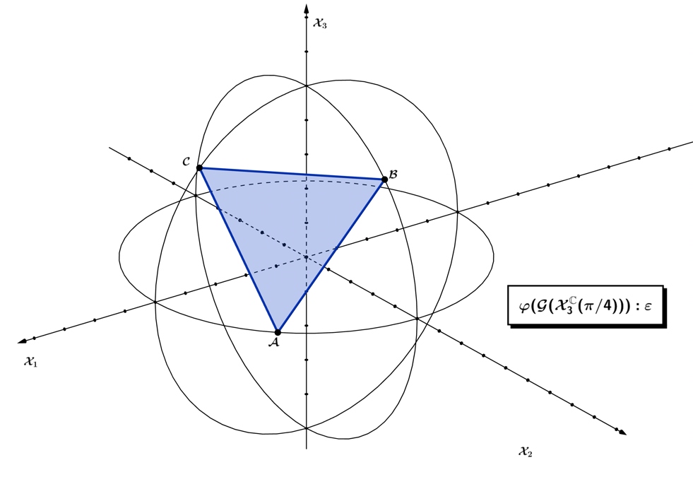
\end{array} (1.2.12) We then compare our original generator G ( X 3 ℂ ) G\left( X_{3}^{\mathbb{C}} \right) i π 4 \frac{i\pi}{4}
ϕ ( G ( X 3 ℂ ( π 4 ) ) : ϵ ) = ( cos ( π 4 ) i s i n ( π 4 ) 0 i s i n ( π 4 ) cos ( π 4 ) 0 0 0 e ( i π 4 ) ) ( A B C ) = ( A c o s ( π 4 ) + i B s i n ( π 4 ) i A s i n ( π 4 ) + B c o s ( π 4 ) C e ( i π 4 ) ) = 1 2 ( i + 1 i + 1 i + 1 ) . \begin{array}{r}
\phi\left( G\left( X_{3}^{\mathbb{C}}\left( \frac{\pi}{4} \right) \right):\epsilon \right) = \begin{pmatrix}
\cos\left( \frac{\pi}{4} \right) & isin\left( \frac{\pi}{4} \right) & 0 \\
isin\left( \frac{\pi}{4} \right) & \cos\left( \frac{\pi}{4} \right) & 0 \\
0 & 0 & e^{\left( \frac{i\pi}{4} \right)}
\end{pmatrix}\begin{pmatrix}
A \\
B \\
C
\end{pmatrix} = \begin{pmatrix}
Acos\left( \frac{\pi}{4} \right) + iBsin\left( \frac{\pi}{4} \right) \\
iAsin\left( \frac{\pi}{4} \right) + Bcos\left( \frac{\pi}{4} \right) \\
Ce^{\left( \frac{i\pi}{4} \right)}
\end{pmatrix} = \frac{1}{\sqrt{2}}\begin{pmatrix}
i + 1 \\
i + 1 \\
i + 1
\end{pmatrix}.
\end{array} (1.2.13) When comparing the mapping, ϕ ( G ( X 3 ℂ ( π 4 ) ) : ϵ ) \phi\left( G\left( X_{3}^{\mathbb{C}}\left( \frac{\pi}{4} \right) \right):\epsilon \right) ϕ ( G ′ ( X 3 ℂ ( π 4 ) ) : ϵ ) , \phi\left( G^{'}\left( X_{3}^{\mathbb{C}}\left( \frac{\pi}{4} \right) \right):\epsilon \right), X 1 / X 2 X_{1}/X_{2} i π 2 \frac{i\pi}{2} ℂ 3 \mathbb{C}^{3} i π 2 \frac{i\pi}{2} e i x e^{ix}
d d x e i x = i e i x , \begin{array}{r}
\frac{d}{dx}e^{ix} = ie^{ix},
\end{array} (1.2.14) coinciding with the result, found by multiplying the ϕ ( G ( X 3 ℂ ( π 4 ) ) : ϵ ) \phi\left( G\left( X_{3}^{\mathbb{C}}\left( \frac{\pi}{4} \right) \right):\epsilon \right) i i
i × 1 2 ( i + 1 i + 1 i + 1 ) = 1 2 ( i − 1 i − 1 i − 1 ) . \begin{array}{r}
i \times \frac{1}{\sqrt{2}}\begin{pmatrix}
i + 1 \\
i + 1 \\
i + 1
\end{pmatrix} = \frac{1}{\sqrt{2}}\begin{pmatrix}
i - \ 1 \\
i - \ 1 \\
i - 1
\end{pmatrix}.
\end{array} (1.2.15) Figure 1.2.1 – The ϕ ( G ( X 3 ℂ ( π 4 ) ) : ϵ ) \phi\left( G\left( X_{3}^{\mathbb{C}}\left( \frac{\pi}{4} \right) \right):\epsilon \right) Figure 1.2.2 – The ϕ ( G ′ ( X 3 ℂ ( π 4 ) ) : ϵ ) \phi\left( G^{'}\left( X_{3}^{\mathbb{C}}\left( \frac{\pi}{4} \right) \right):\epsilon \right) We plot both results ∈ ℂ 3 \in \mathbb{C}^{3} Figures 1.2.1-2 U ( 3 ) U(3) G ( X 3 ℂ ) G\left( X_{3}^{\mathbb{C}} \right) G ′ ( X 3 ℂ ) G^{'}\left( X_{3}^{\mathbb{C}} \right) ϕ ( G ′ ( X 3 ℂ ( π 4 ) ) : ϵ ) \phi\left( G^{'}\left( X_{3}^{\mathbb{C}}\left( \frac{\pi}{4} \right) \right):\epsilon \right) ϕ ( G ( X 3 ℂ ( π 4 ) ) : ϵ ) \phi\left( G\left( X_{3}^{\mathbb{C}}\left( \frac{\pi}{4} \right) \right):\epsilon \right) ∈ ℂ 3 \in \mathbb{C}^{3} ‖ 𝐳 ‖ \left\| \mathbf{z} \right\|
‖ ϕ ( G ( X 3 ℂ ( π 4 ) ) : ϵ ) ‖ = | 1 2 + i 2 | + | 1 2 + i 2 | + | 1 2 + i 2 | = 3 \begin{array}{r}
\left\| \phi\left( G\left( X_{3}^{\mathbb{C}}\left( \frac{\pi}{4} \right) \right):\epsilon \right) \right\| = \sqrt{\left| \frac{1}{\sqrt{2}} + \frac{i}{\sqrt{2}} \right| + \left| \frac{1}{\sqrt{2}} + \frac{i}{\sqrt{2}} \right| + \left| \frac{1}{\sqrt{2}} + \frac{i}{\sqrt{2}} \right|} = \sqrt{3}
\end{array} (1.2.16) is equal to
‖ ϕ ( G ′ ( X 3 ℂ ( π 4 ) ) : ϵ ) ‖ = | i 2 − i 2 | + | i 2 − 1 2 | + | i 2 − 1 2 | = 3 . \begin{array}{r}
\left\| \phi\left( G^{'}\left( X_{3}^{\mathbb{C}}\left( \frac{\pi}{4} \right) \right):\epsilon \right) \right\| = \sqrt{\left| \frac{i}{\sqrt{2}} - \frac{i}{\sqrt{2}} \right| + \left| \frac{i}{\sqrt{2}} - \frac{1}{\sqrt{2}} \right| + \left| \frac{i}{\sqrt{2}} - \frac{1}{\sqrt{2}} \right|} = \sqrt{3}.
\end{array} (1.2.17)