1.6.6 The Alternating Harmonic Series and its Inverse Analog

We return to the field ${S_{H} = D}_{X}^{- 1}X$, from the last sec­tion, which was equiv­a­lent to the outer prod­uct of el­e­ments in the two series

whose matrix $S_{H}$, we again show, as

As seen in the array above, the in­verse al­ter­nat­ing har­mon­ic series is rep­re­sent­ed in the first row, and the al­ter­nat­ing nat­ur­al num­bers are in the first column, which relate by the equiv­a­lence ex­pres­sion,

We know that the har­mon­ic series di­verges, albeit very slowly, but the al­ter­nat­ing har­mon­ic series con­verges to $\ln(2)$

which has par­tial sums equal to

where the func­tion $\Phi(z,s,a)$, is the Lerch tran­scen­dent, de­fined as the sum­ma­tion

with the in­te­gral rep­re­sen­ta­tion

The $\Phi(z,s,\alpha)$ func­tion en­com­pass­es many famous func­tions that play a cen­tral role in math­e­mat­i­cal analy­sis, and ar­guably the most famous of them is the Rie­mann zeta func­tion $\zeta(s),$which is equiv­a­lent to $\Phi(1,s,0)$

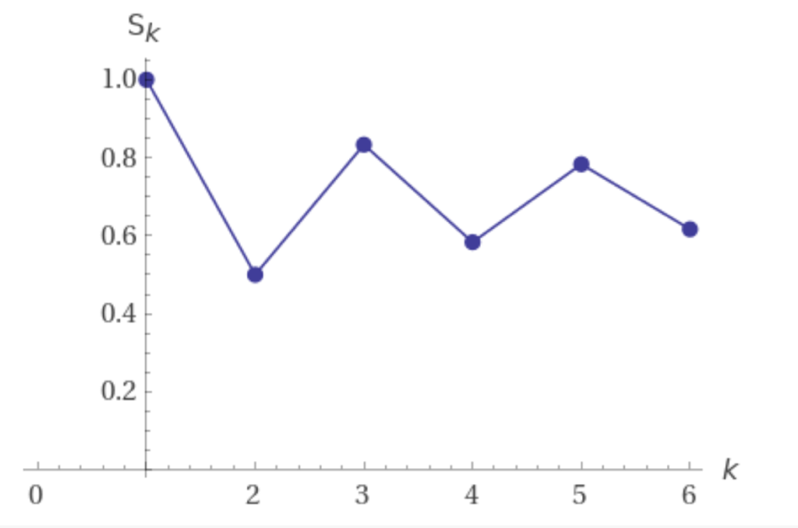
Plot­ting par­tial sums, $S_{k}$, for the func­tion $( - 1)^{n + 1}\Phi( - 1,1,n + 1) + \ln(2)$ in Figure 1.6.15, we can see that these are trend­ing to the con­ver­gence value of $\ln(2) \approx 0.6931$.

The par­tial sum of the al­ter­nat­ing har­mon­ic series, can also be ex­pressed in the form of the Lerch tran­scen­dent and $\ln(2)$

and it is in­trigu­ing that the sum of two in­fi­nite series con­verges to our finite par­tial AHS sum, where the Lerch tran­scen­dent is de­fined, as $\Phi( - 1,1,n + 1)$

and our par­tial sum func­tion equals

Ex­pand­ing this sum­ma­tion

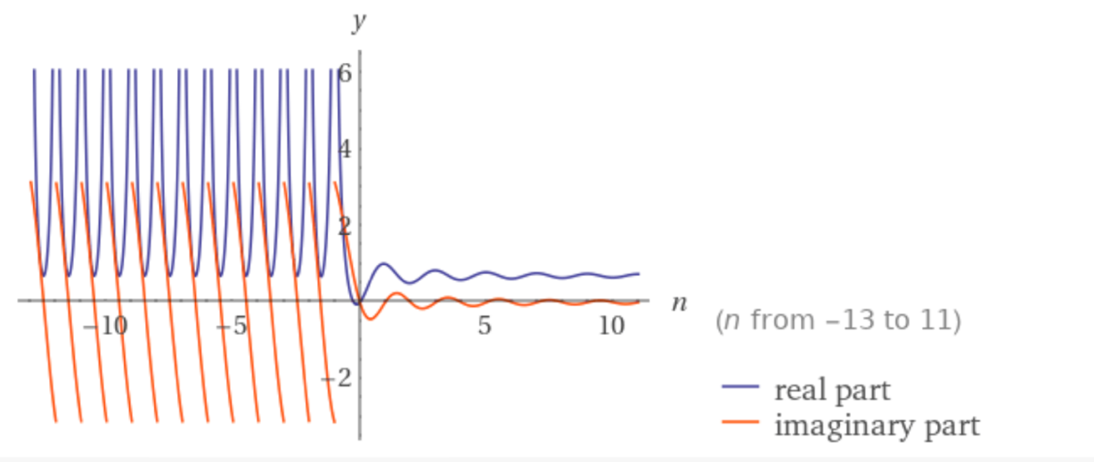
it is easy to see the log­a­rithm func­tion in the sum­ma­tion terms. The Lerch tran­scen­dent ex­tends the al­ter­nat­ing har­mon­ic series to the com­plex plane and beyond the "zero-point", by taking the par­tial sums of the al­ter­nat­ing har­mon­ic series and making the func­tion con­tin­u­ous, as seen in the figure below.

The now fa­mil­iar in­verse har­mon­ic series or al­ter­nat­ing nat­ur­al num­bers,

has a closed form for its par­tial sums $S_{j},$in the form

but for the limit, as $n \rightarrow \infty$, $S_{j}$ ap­pears to be di­ver­gent

It turns out the series is reg­u­lar­iz­able, where­by using the Borel reg­u­lar­iza­tion tech­nique, we find $\frac{1}{4}$ for its result

Like the har­mon­ic num­bers $H_{k}$, the in­verse har­mon­ic num­bers are com­posed of par­tial sums of the nat­ur­al number set $\mathbb{N}$. We choose the no­ta­tion $N_{k}$, to rep­re­sent par­tial sums of the nat­ur­al num­bers, and $H_{k}^{\pm}$ for par­tial sums of the al­ter­nat­ing har­mon­ic series. And a simple closed form also exists for $N_{k}$, as

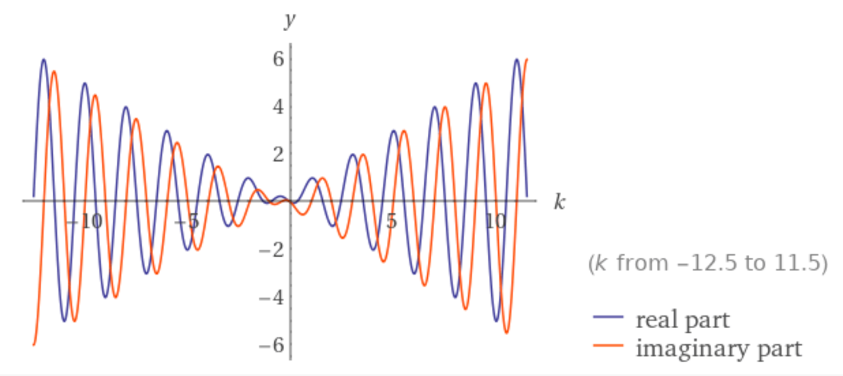
Fur­ther defin­ing par­tial sums of al­ter­nat­ing nat­ur­al num­bers as $N_{k}^{\pm}$, they have the very beau­ti­ful prop­er­ty of os­cil­lat­ing be­tween pos­i­tive and neg­a­tive values for each suc­ces­sive it­er­a­tion in their par­tial sum series. By ac­cept­ing that $k$ is not re­strict­ed to the nat­ur­al num­bers, and in­stead that $k\in \mathbb{R}$, we find the ap­peal­ing plot in Figure 1.6.17. The image shows the real valued por­tion of the plot forms a sym­met­ric wave­form em­a­nat­ing out from the value $k = - \frac{1}{2}$, while the imag­i­nary values also os­cil­late, but the wave­form is not sym­met­ric, acting like an odd func­tion. Both of the wave­forms will main­tain con­sis­tent wave­lengths, while steadi­ly grow­ing or shrink­ing in am­pli­tude, de­pend­ing on their move­ment toward or from the value $k = 0.$Given its wave­like ap­pear­ance, it is not sur­pris­ing that $N_{k}^{\pm}$, for $k\in \mathbb{R}$, can be ex­pressed using sine and cosine func­tions, as

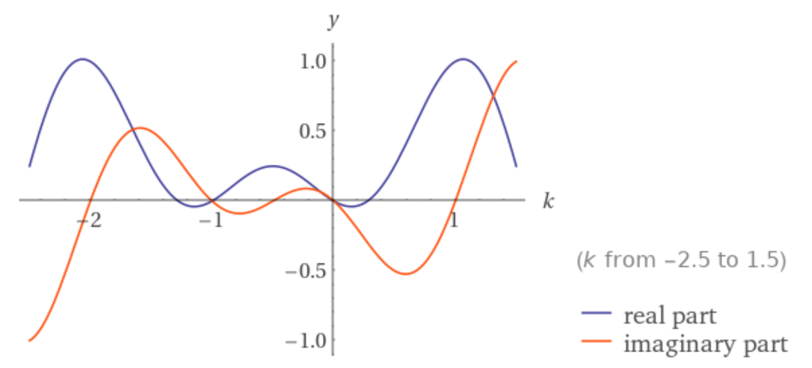
Zoom­ing in on the figure above to the area just to the left of the origin, re­veals a very beau­ti­ful part of the func­tion (Figure 1.6.18), where at­ten­tion should be di­rect­ed to the point $k = - \frac{1}{2},$which solv­ing the par­tial sum equa­tion for the in­verse har­mon­ic number $N_{\left( - \frac{1}{2} \right)}^{\pm}$, we find that it equals our Borel reg­u­lar­iza­tion value of $\frac{1}{4},$

So, the center of sym­me­try at $N_{\left( - \frac{1}{2} \right)}^{\pm} = \frac{1}{4}$, for the real wave­form of the func­tion $N_{k}^{\pm}$, is due to an­a­lyt­ic con­tin­u­a­tion, and this is a process that we will ex­plore thor­ough­ly for other func­tions in the next book. The reg­u­lar­iza­tion of the $N_{k}^{\pm}$ series, makes it pos­si­ble to con­sid­er the reg­u­lar­iza­tion of the entire outer-prod­uct array from Eq. 1.6.181, which was formed by the al­ter­nat­ing nat­ur­al number series and the al­ter­nat­ing har­mon­ic series

So, we can con­sid­er the reg­u­lar­iza­tion of the $S_{H}$ outer-prod­uct array as the sum­ma­tion of the reg­u­lar­ized al­ter­nat­ing in­verse har­mon­ic/nat­ur­al number series

mul­ti­plied by each value in the al­ter­nat­ing har­mon­ic series as we pro­ceed right­ward by column, re­sult­ing in the series, which con­verges to $\frac{\ln(2)}{4}$

This leads to the fol­low­ing de­f­i­n­i­tion for the outer-prod­uct reg­u­lar­iza­tion:

De­f­i­n­i­tion (1.6.202) – The Reg­u­lar­ized In­fi­nite Outer-Prod­uct Sum­ma­tion is a sum of el­e­ments, from two or more in­fi­nite series, that con­verges to a value or a func­tion, where at least one of the series that forms this outer-prod­uct is di­ver­gent but reg­u­lar­iz­able, and the other series(s) may or may not be an in­de­pen­dent­ly con­ver­gent series.

Let $\mathcal{R}(A)$, denote a reg­u­lar­ized sum­ma­tion for an in­fi­nite series of el­e­ments, $a_{k}$,

which can form an outer prod­uct with an­oth­er in­fi­nite series or func­tion ex­pan­sion, $B$, that may or may not con­verge in­de­pen­dent­ly. For an in­de­pen­dent­ly con­ver­gent series, $B$, the outer prod­uct with $\mathcal{R}(A)$, is

having the fol­low­ing Reg­u­lar­ized In­fi­nite Outer-Prod­uct Sum­ma­tion

and for a di­ver­gent but reg­u­lar­iz­able series $B$, this forms the outer prod­uct with $\mathcal{R}(A)$,

having the Reg­u­lar­ized In­fi­nite Outer-Prod­uct Sum­ma­tion

By having a de­f­i­n­i­tion for the reg­u­lar­ized in­fi­nite outer-prod­uct sum­ma­tion, we can ex­press the pre­vi­ous ex­am­ple for the two al­ter­nat­ing har­mon­ic series as

which has the sum­ma­tion

To demon­strate a reg­u­lar­ized in­fi­nite outer-prod­uct sum­ma­tion that con­verges to a func­tion, we can use a vari­able $z\in \mathbb{C}$, to con­sid­er the outer-prod­uct

where the right­hand sum will con­verge to $\ln(z)$, for $|z - 1| < 1 \land z = 2$, and the reg­u­lar­ized in­fi­nite outer-prod­uct sum­ma­tion will con­verge to the fol­low­ing func­tion

The Basel prob­lem stumped many math­e­mati­cians after first being pro­posed by Pietro Men­goli in 1650, where the prob­lem was to pre­cise­ly de­ter­mine the sum­ma­tion of the squared rec­i­p­ro­cals of the nat­ur­al num­bers, de­fined as the in­fi­nite sum

It was ul­ti­mate­ly solved by Leon­hard Euler¹ in 1734, when he found the sum equaled $\pi^{2}/6$; a sur­pris­ing result, given the pres­ence of $\pi$. The os­cil­la­tions that we have noted in our par­tial sum­ma­tion of the in­verse al­ter­nat­ing har­mon­ic num­bers, hint at the pres­ence of cir­cu­lar phe­nom­e­non in this series as well. Taking a closer look at the equa­tion,

we have that, $( - 1)^{k + 1}$& $2k( - 1)^{k}$ are al­ge­bra­ic forms of the fol­low­ing com­plex ex­po­nen­tial func­tions

lead­ing to the equiv­a­lent ex­pres­sion,

and can be fur­ther sim­pli­fied to

Like the Basel sum­ma­tion, we find the pres­ence of not only $\pi$ lurk­ing in the in­verse al­ter­nat­ing har­mon­ic num­bers, but also the com­plex ex­po­nen­tial func­tion. The har­mon­ic series, we have briefly dis­cussed in this sec­tion, plays an im­por­tant role in analy­sis, pro­vid­ing the ground­work for the next book, ul­ti­mate­ly taking us to the heart of prime number theory.

1. Euler, Leonard, "De summis se­rierum rec­i­p­ro­carum", Com­men­tarii Acad­e­mi­ae Sci­en­tiarum Pet­ro­pol­i­tanae, Volume 7:123-134, 1735