Masteries · Jason GlowneyArithmoí Book 1

Masteries

1.3.2 The Space of Angles ∈ℂ\in \mathbb{C}

Con­sid­er­ing geo­met­ric man­i­folds as open sets re­sid­ing in a higher-di­men­sion­al angle space, as op­posed to a higher-di­men­sion­al Eu­clid­ean space, af­fords pre­cise clar­i­ty re­gard­ing how these geome­tries in­ter­re­late. Real-valued dis­tances, like the xx and yy co­or­di­nate axes in the two-di­men­sion­al Carte­sian plane, typ­i­cal­ly rep­re­sent our first for­ma­tive ex­po­sure to geo­met­ric spaces. When we give pri­or­i­ty to an angle space ∈ℂ\in \mathbb{C}, in­stead of the Carte­sian space geom­e­try ∈ℝ\in \mathbb{R}, a more in­flu­en­tial mean­ing and depth is ren­dered con­cern­ing geo­met­ric spaces. When con­sid­er­ing the real-valued ex­pres­sion of the circle

x2+y2=r,\begin{array}{r} x^{2} + y^{2} = r, \end{array}
(1.3.3)

and its trigono­met­ric form

rcos2(α)+rsin2(α)=r,\begin{array}{r} {rcos}^{2}(\alpha) + {rsin}^{2}(\alpha) = r, \end{array}
(1.3.4)

we have so­lu­tions for Eq. 1.3.4 for any chosen angle α∈ℝ\alpha\in \mathbb{R}. The single angle ar­gu­ment in the trigono­met­ric ex­pres­sion of the circle im­plies the two di­men­sions of the Carte­sian co­or­di­nate system. These trigono­met­ric sine and cosine func­tions are de­pen­dent on ∠α\angle\alpha. At the same time, these func­tions are in­ter­de­pen­dent, and the give and take that de­fines their cor­re­lat­ed values en­sures the circle's dis­tance metric holds in­vari­ant. We con­sid­er the ex­po­nen­tial series for a single angle value XX

eX=∑n=0∞Xnn!=X00!+X11!+X22!+X33!+X44!+…,\begin{array}{r} e^{X} = \sum_{n = 0}^{\infty}\frac{X^{n}}{n!} = \frac{X^{0}}{0!} + \frac{X^{1}}{1!} + \frac{X^{2}}{2!} + \frac{X^{3}}{3!} + \frac{X^{4}}{4!} + \ldots, \end{array}
(1.3.5)

which can be sep­a­rat­ed into odd and even el­e­ments to define the cosh⁡(X)\cosh(X) and sinh⁡(X)\sinh(X) func­tions

eX={1+X22!+X44!+…}+{X11!+X33!+X55!+…}=cosh⁡(X)+sinh⁡(X).\begin{array}{r} e^{X} = \left\{ 1 + \frac{X^{2}}{2!} + \frac{X^{4}}{4!} + \ldots \right\} + \left\{ \frac{X^{1}}{1!} + \frac{X^{3}}{3!} + \frac{X^{5}}{5!} + \ldots \right\} = \cosh(X) + \sinh(X). \end{array}
(1.3.6)

Math­e­mat­i­cal­ly, it has been known since the time of Euler, al­low­ing XX to be imag­i­nary-valued leads to the for­mu­la we all hold dear

eiX={1−X22!+X44!−…},   {iX11!−iX33!+iX55!−…}=cos⁡(X)+isin(X).\begin{array}{r} e^{iX} = \left\{ 1 - \frac{X^{2}}{2!} + \frac{X^{4}}{4!} - \ldots \right\},\ \ \ \left\{ \frac{iX^{1}}{1!} - \frac{iX^{3}}{3!} + \frac{iX^{5}}{5!} - \ldots \right\} = \cos(X) + {isin}(X). \end{array}
(1.3.7)

In plain sight, with the ex­am­ples above, is an exact cor­re­spon­dence be­tween the unit circle and the unit hy­per­bo­la. This cor­re­spon­dence boils down to their re­spec­tive ori­en­ta­tions in the angle-ar­gu­ment space ∈ℂ\in \mathbb{C}. These ex­po­nen­tial series and their trigono­met­ric func­tions are sub­sets of the same higher-di­men­sion­al com­plex angle space.

Figure
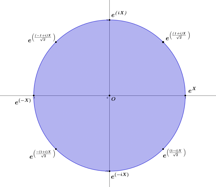
Figure 1.3.6 – The Angle Space Ring.

For the two-di­men­sion­al ex­am­ple, the com­plex angle space rep­re­sents a com­plex unit circle nested in the space of the angle vari­ables. Through the ex­po­nen­tial map­ping, each point on its bound­ary rep­re­sents a unique man­i­fold, ad­mit­ting angles ∈ℂ\in \mathbb{C}. We can refer to this as the Angle Space Ring, shown in Figure 1.3.6, where com­plex-valued angles are point rep­re­sen­ta­tions on its bound­ary. The ring, by way of the ex­po­nen­tial map­ping, gives rise to unique ex­po­nen­tial func­tions, where the figure's ex­am­ples are ori­ent­ed along the imag­i­nary-axis (e(iπX2),e(3iπX2))\left( e^{\left( \frac{i\pi X}{2} \right)},e^{\left( \frac{3i\pi X}{2} \right)} \right), the real-axis (e(2iπX),e(iπX))\left( e^{(2i\pi X)},e^{(i\pi X)} \right), and the as­ymp­tot­ic axes (e(iπX4),e(3iπX4),e(5iπX4) ,e(7iπX4))\left( e^{\left( \frac{i\pi X}{4} \right)},e^{\left( \frac{3i\pi X}{4} \right)},e^{\left( \frac{5i\pi X}{4} \right)}\ ,e^{\left( \frac{7i\pi X}{4} \right)} \right), all rep­re­sent­ing points on the Angle Space Ring.

Along pos­i­tive real and imag­i­nary axes, the ex­po­nen­tial map­ping of the points e(2iπX),e(iπX2)e^{(2i\pi X)},e^{\left( \frac{i\pi X}{2} \right)} is straight­for­ward, giving rise to the subset man­i­folds eiXe^{iX} and eXe^{X}. For subset man­i­folds, the angle ar­gu­ments are rep­re­sent­ed by points on the ring be­tween axes, taking on com­plex-valued angles of the form ∠=X(eiβ):X,β∈ℝ\angle = X\left( e^{i\beta} \right):X,\beta\in \mathbb{R}. Using the ex­am­ple for the point lo­cat­ed on the right at e(iπX4),e^{\left( \frac{i\pi X}{4} \right)}, β=iπ4\beta = \frac{i\pi}{4} ra­di­ans, re­sult­ing in a man­i­fold de­fined by the ex­po­nen­tial map­ping

eX∙e(iπ4)=eiX=eX(12 + i2).\begin{array}{r} e^{X \bullet e^{\left( \frac{i\pi}{4} \right)} =}e^{\sqrt{i}X} = e^{X\left( \frac{1}{\sqrt{2}}\ + \ \frac{i}{\sqrt{2}} \right)}. \end{array}
(1.3.8)

Com­plex-Angle Space is the for­mal­ly de­fined, as fol­lows:

De­f­i­n­i­tion (1.3.9) – The Com­plex-Angle Space is a com­plex nn-di­men­sion­al angle space Bn\mathrm{B}_{n}, which is the set that con­tains all the subset Lie groups G, with angles of the form Xn(eiβn)X^{n}\left( e^{i\beta_{n}} \right), rep­re­sent­ing the tan­gent space of the Lie group G=exp⁡(Xn(eiβn))G = \exp\left( X^{n}\left( e^{i\beta_{n}} \right) \right), Xn∈ℝnX^{n} \in \mathbb{R}^{n}, and all tan­gent spaces Xn(eiβn)X^{n}\left( e^{i\beta_{n}} \right) lay on the bound­ary ∂Bn.\partial \mathrm{B}_{n}.

De­f­i­n­i­tion (1.3.10) – Let G(X),G(Y)⊂BG(X),G(Y) \subset \mathrm{B} be ar­bi­trary Lie groups, rep­re­sent­ing closed sub­sets of the Com­plex-Angle Space B𝐧.\mathbf{\mathrm{B}}_{\mathbf{n}}. 𝛀:𝐆(𝐗)→𝐆(𝐘)\boldsymbol{\Omega}:\mathbf{G}\left( \mathbf{X} \right)\rightarrow \mathbf{G}\left( \mathbf{Y} \right) is a bi­jec­tive and con­tin­u­ous map­ping that takes the Lie group G(Xn)∈Bn{G(X}^{n}) \in \mathrm{B}_{n} to G(Yn)∈BnG\left( Y^{n} \right) \in \mathrm{B}_{n},

Ω:G(Xn)→G(Yn)∈B(n,ℂ).\begin{array}{r} \Omega:G\left( X^{n} \right) \rightarrow {G(Y}^{n}) \in \mathrm{B}\left( n,\mathbb{C} \right). \end{array}

We define the func­tion map­ping Ω:G(Xn)\Omega:G\left( X^{n} \right), for a chosen com­plex angle trans­for­ma­tion eiβne^{i\beta_{n}}

Ω:G(Xn)=G(Xn∙eiβn),\begin{array}{r} \Omega:G\left( X^{n} \right) = G\left( X^{n} \bullet e^{i\beta_{n}} \right), \end{array}

for Xn∙eiβnX^{n} \bullet e^{i\beta_{n}}, rep­re­sent­ing the el­e­ment-to-el­e­ment mul­ti­plica­tive prod­uct of the two n×nn \times n ma­tri­ces.

For the n=1n = 1 di­men­sion­al case, the map­ping Ω:G(Xn)→G(Yn)\Omega:G\left( X^{n} \right) \rightarrow {G(Y}^{n}) is straight­for­ward, ap­pre­ci­at­ed for three-di­men­sion­al map­ping ex­am­ple

Ω:G(X13ℂ)→G(X13ℝ),\begin{array}{r} \Omega:{G(X}_{1}^{3\mathbb{C}}) \rightarrow {G(X}_{1}^{3\mathbb{R}}), \end{array}
(1.3.11)

for G(X13ℂ){G(X}_{1}^{3\mathbb{C}}), a gen­er­a­tor from the D3ℂD_{3\mathbb{C}} di­he­dral group, and G(X13ℝ){G(X}_{1}^{3\mathbb{R}}), a gen­er­a­tor from the D3ℝD_{3\mathbb{R}} group. We set β=−π2\beta = \frac{- \pi}{2}, while re­call­ing the func­tion X∘βX \circ \beta rep­re­sents the re­sult­ing matrix formed by the el­e­ment-to-el­e­ment mul­ti­pli­ca­tion prod­ucts (xj,k∙βj,k(x_{j,k} \bullet \beta_{j,k}), find­ing

Ω:G(X3)=G(X3∘eiβ3)=exp⁡((ix10000ix10ix10)∘(e−iπ20000e−iπ20e−iπ20))=exp⁡(X13ℝ)=G(X13ℝ).\begin{array}{r} \Omega:G\left( X^{3} \right) = G\left( X^{3} \circ e^{i\beta_{3}} \right) = \exp\left( \begin{pmatrix} ix_{1} & 0 & 0 \\ 0 & 0 & ix_{1} \\ 0 & ix_{1} & 0 \end{pmatrix} \circ \begin{pmatrix} e^{- \frac{i\pi}{2}} & 0 & 0 \\ 0 & 0 & e^{- \frac{i\pi}{2}} \\ 0 & e^{- \frac{i\pi}{2}} & 0 \end{pmatrix} \right) = \exp\begin{array}{r} \left( X_{1}^{3\mathbb{R}} \right) = {G(X}_{1}^{3\mathbb{R}}). \end{array} \end{array}
(1.3.12)

The di­he­dral forms of the Lie groups that we have been work­ing with belong to the gen­er­al linear group GL(3,ℂ)∈ℂ3GL\left( 3,\mathbb{C} \right) \in \mathbb{C}^{3}

G(X3∘eiβ3)∈GL(3,ℂ).\begin{array}{r} G\left( X^{3} \circ e^{i\beta_{3}} \right) \in GL\left( 3,\mathbb{C} \right). \end{array}
(1.3.13)

The Ω(X)\Omega(X) map­ping is bi­jec­tive, and given that these groups are all con­tin­u­ous, the topo­log­i­cal spaces G(Xn),G(Yn)G\left( X^{n} \right),{G(Y}^{n}) are home­o­mor­phic to one an­oth­er.

The­o­rem (1.3.14) – For any two topo­log­i­cal spaces of the form G(X),G(Y)G(X),G(Y), lo­cat­ed on the bound­ary ∂B\partial \mathrm{B} in com­plex-angle space, there is a ho­mo­mor­phism be­tween G(X)G(X) and G(Y)G(Y).

Proof – The map­ping Ω:G(X)→G(Y)\Omega:G(X) \rightarrow G(Y) of any two func­tions of the form G(X),G(Y)G(X),G(Y) lo­cat­ed on the bound­ary ∂B\partial B in com­plex-angled space is a bi­jec­tive (one-to-one) and con­tin­u­ous map­ping, and there is an in­verse map­ping Ω−1:G(Y)→G(X)\Omega^{- 1}:G(Y) \rightarrow G(X) for any map­ping Ω:G(X)→G(Y)\Omega:G(X) \rightarrow G(Y), that is also bi­jec­tive and con­tin­u­ous. The map­ping,

Ω:G(Xn)=G(Xn∘eiβn)=G(Yn),\begin{array}{r} \Omega:G\left( X^{n} \right) = G\left( X^{n} \circ e^{i\beta_{n}} \right) = G\left( Y^{n} \right), \end{array}

maps each el­e­ment of XnX^{n} to YnY^{n} bi­jec­tive­ly. For every map­ping G(Xn∘eiβn)G\left( X^{n} \circ e^{i\beta_{n}} \right) there is an in­verse map­ping,

Ω−1:G(Yn)=G(Yn∘ei(−β)n)=G(Xn),\begin{array}{r} \Omega^{- 1}:G\left( Y^{n} \right) = G\left( Y^{n} \circ e^{i( - \beta)_{n}} \right) = G\left( X^{n} \right), \end{array}

by way of com­plex con­ju­ga­tion eiβn=ei(−β)n\overline{e^{i\beta_{n}}} = e^{i( - \beta)_{n}}, which maps G(Yn)G\left( Y^{n} \right) back to G(Xn)G\left( X^{n} \right).

 □\begin{array}{r} \ \square \end{array}
Figure
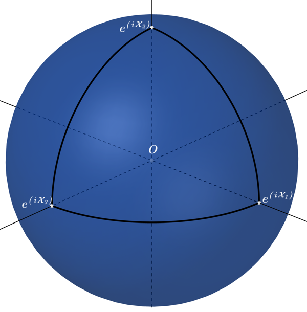
Figure 1.3.7 – Start­ing angle trans­for­ma­tion Ω:G3ℂ(X1+X2+X3)→G3ℝ(X1+X2,+X3)\Omega:G^{3\mathbb{C}}\left( X_{1} + X_{2} + X_{3} \right) \rightarrow G^{3\mathbb{R}}\left( X_{1} + X_{2}, + X_{3} \right).

To frame the math­e­mat­ics in simple terms, one can choose an angle in com­plex space to rotate one man­i­fold to an­oth­er through an angle space trans­for­ma­tion. Con­cern­ing the di­he­dral form's Lie groups, these can be rep­re­sent­ed on the sphere in com­plex-angle space, which is anal­o­gous to the two-di­men­sion­al rep­re­sen­ta­tion from Figure 1.3.6. Using the U(3)U(3) group ex­am­ple, we find it can be ro­tat­ed to the hy­per­bol­ic form by the map­ping,

Ω:G3ℂ(X1+X2+X3)→G3ℝ(X1+X2,+X3),\begin{array}{r} \Omega:G^{3\mathbb{C}}\left( X_{1} + X_{2} + X_{3} \right) \rightarrow G^{3\mathbb{R}}\left( X_{1} + X_{2}, + X_{3} \right), \end{array}
(1.3.15)

by set­ting β1,β2,β3=−π2\beta_{1},\beta_{2},\beta_{3} = \frac{- \pi}{2}, then eval­u­at­ing the al­ge­bra map­ping

Ω:G3ℂ(X1+X2+X3)=G3ℂ(X1∘eiβ1,X2∘eiβ2,X3∘eiβ3)=G3ℝ(X1+X2,+X3).\begin{array}{r} \Omega:G^{3\mathbb{C}}\left( X_{1} + X_{2} + X_{3} \right) = G^{3\mathbb{C}}\left( X_{1} \circ e^{i\beta_{1}},X_{2} \circ e^{i\beta_{2}},X_{3} \circ e^{i\beta_{3}} \right) = G^{3\mathbb{R}}\left( X_{1} + X_{2}, + X_{3} \right). \end{array}
(1.3.16)

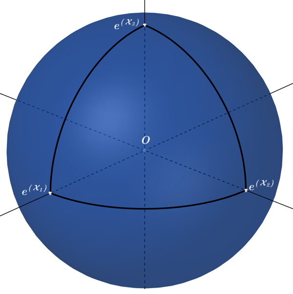
A geo­met­ric vi­su­al­iza­tion of the angle trans­for­ma­tion from above can be shown by con­nect­ing points rep­re­sent­ing the per­mu­ta­tion gen­er­a­tors from the G3ℂG^{3\mathbb{C}} group (eiX1,eiX2,eiX3)\ \left( e^{iX_{1}},e^{iX_{2}},e^{iX_{3}} \right), with cir­cu­lar arcs on the com­plex-angled space sphere. For β1,β2,β3=−iπ2\beta_{1},\beta_{2},\beta_{3} = \frac{- i\pi}{2}, a clock­wise ro­ta­tion occurs for each G3ℂG^{3\mathbb{C}}per­mu­ta­tion gen­er­a­tor by −iπ2\frac{- i\pi}{2} ra­di­ans. By taking eiXj→eXje^{iX_{j}} \rightarrow e^{X_{j}}, seen in Fig­ures 1.3.7-8, the imag­i­nary-valued gen­er­a­tors lo­cat­ed on the ver­tices of the tri­an­gle have each ro­tat­ed by −iπ2\frac{- i\pi}{2} in their re­spec­tive planes, and arrive at their co­in­cid­ing real-valued gen­er­a­tor forms.

Figure
Figure 1.3.8 – Re­sult­ing angle trans­for­ma­tion, Ω:G3ℂ(X1+X2+X3)→G3ℝ(X1+X2,+X3)\Omega:G^{3\mathbb{C}}\left( X_{1} + X_{2} + X_{3} \right) \rightarrow G^{3\mathbb{R}}\left( X_{1} + X_{2}, + X_{3} \right).