The last two sections revealed how the tangent space and Lie algebras are connected, that being, the group derivative is a phase shift that depends on the Lie algebra of the said specific group. Algebraic layers exist beneath the tangent space, which will be considered in this section as we push deeper into the functional spaces. In the last section, we considered the following group derivative operation
(1.2.166)
which served to conceptualize the tangent space and its geometric arrangement to that of the Lie algebra. The derivative operation represents a velocity in the group space, which we denote as , and set it equal to from the example above
(1.2.167)
Matrix multiplication of the group by the Lie algebra reveals the phase-shift and dynamical trigonometric dependency conferred from this subgroup onto , as seen in the concise derivative form
(1.2.168)
which is equivalent to in a phase-shifted form
(1.2.169)
As we are aware, the group is the exponential mapping of its Lie algebra , and this relationship holds for with its Lie algebra . The matrix logarithm represents the inverse of the exponential mapping, and evaluating the logarithm of yields the Lie algebra we arrived at via the tangent space consideration
(1.2.170)
This should not be considered solely as the phase-shifted algebra, but instead as a phase-shifted group representing the tangent space velocity,
(1.2.171)
The tangent velocity is equal to the sum of its Lie algebra and the phase-shift dependency , which is conferred on by the subalgebra denoted as
(1.2.172)
which after setting , becomes
(1.2.173)
The algebra results from the evaluation of the matrix logarithm of a matrix logarithm function
(1.2.174)
and if we were to carry out repeated iterative matrix logarithm functions indefinitely
(1.2.175)
the resulting algebra will converge to the approximate form
(1.2.176)
Perhaps more striking is that all numbers, except for one, zero, , and any numbers related to in the form appear to converge to either
(1.2.177)
for , or to
(1.2.178)
for . The intuition behind these two numbers is that they are the two solutions to the equation
(1.2.179)
which means they also represent the two solutions to
(1.2.180)
given that for the defined
(1.2.181)
The numbers , are related to the multivalued Lambert function, also known as the product log function, which, for , have the property that the expression
(1.2.182)
holds if and only if for some integer , the following expression holds
(1.2.183)
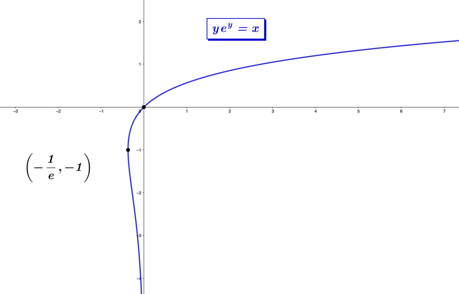
where is conversely related to the function. For real number values, the expression
(1.2.184)
has solutions for if . This endpoint at occurs when ,
(1.2.185)
and the possible solutions for are well-demonstrated in the expression's plot in the Figure 1.2.7.
Figure 1.2.7 – The expression , plotted.
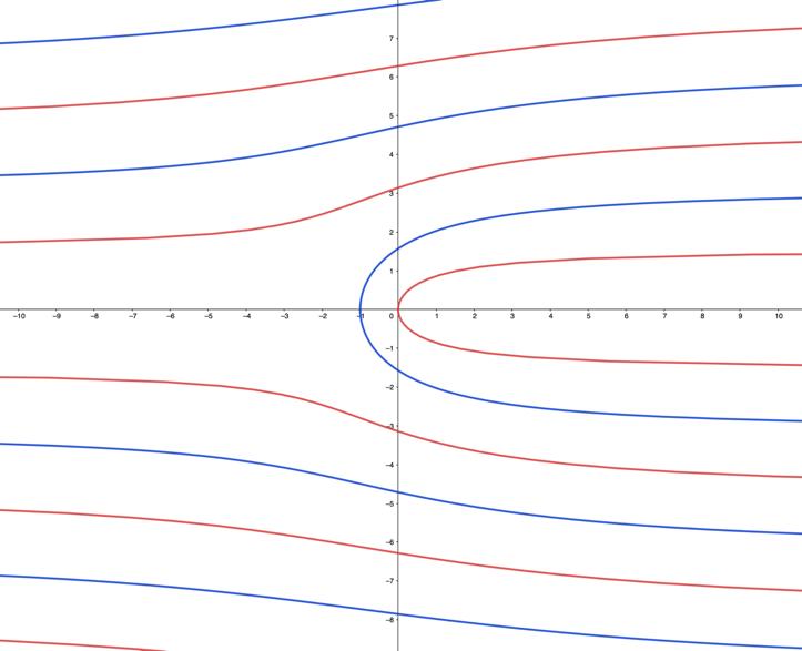
We can consider the range of the Lambert function in the complex plane by setting , for , to express , as
(1.2.186)
and rearrange the expression
(1.2.187)
where one portion of the result is real, and the other part is imaginary. The imaginary portion will equal zero when
(1.2.188)
and the real branches of the Lambert function's range are found by solving for the variable
(1.2.189)
Similarly, by setting the real portion equal to zero, we find the imaginary branches in the range are
(1.2.190)
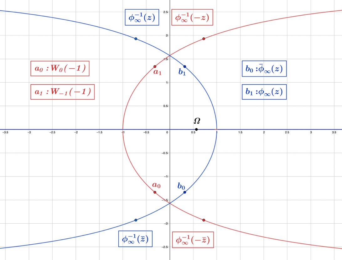
We plot the range of the Lambert function in Figure 1.2.8, where imaginary branches are shown in red, and the real branches are shown in blue. Returning to the numbers and , we find they are endowed with the extraordinary property that they maintain the same result for their proper logarithm and exponential mappings
(1.2.191)
(1.2.192)
implying these numbers represent a meeting point in complex space of the exponential and logarithm functions. These numbers can be expressed as equivalent to the following negative-valued functions
(1.2.193)
(1.2.194)
Figure 1.2.8 – The function's range shows real branches in blue and imaginary branches in red.
To further consider the unique properties of these numbers, we start by finding the polar form of
(1.2.195)
where the radial component is , and since , the angle argument is found by the inverse tangent function
(1.2.196)
What stands out at first glance in the approximated polar form
(1.2.197)
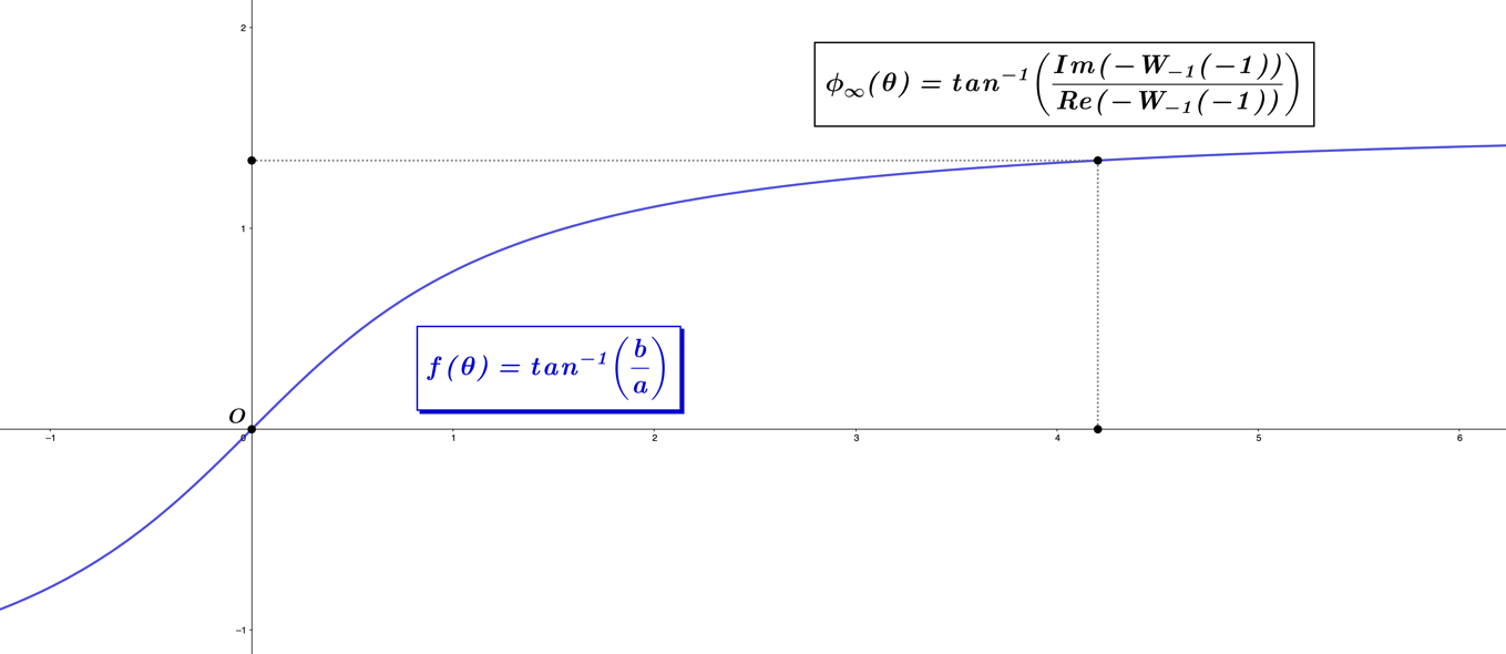
is that is equal to the imaginary part of the complex number, ,
(1.2.198)
Figure 1.2.7 – A plot of the function , with the point
coinciding with the polar angle argument resultdenoted.
We consider the function by looking at its plot Figure 1.2.7 for complex numbers , and . The point with coordinates , coinciding with the angle variable is discerned
(1.2.199)
Evaluation of the radial component for , yields
(1.2.200)
having the unique property that its logarithm equals the real part of the function
(1.2.201)
When combined with the polar form's angle, this means that can be expressed as the exponential product of its real and imaginary parts
(1.2.202)
and given that
(1.2.203)
we have a better mathematical understanding of how Concerning the expression , and the Lambert function, the numbers and represent the two conforming and conjugately-related solutions for
(1.2.204)
(1.2.205)
meaning these are the two solutions of the expression The well-known omega constant defines the unique real number solution to the expression
(1.2.206)
representing the Lambert function with an approximated value
(1.2.207)
Analogous to and the following -related identities are a direct consequence of
(1.2.208)
(1.2.209)
With the identities in mind, we define the algebra as the indefinitely repeated negative matrix logarithm function
(1.2.210)
which interestingly, "converges" to two alternating conjugately-related points composed by the algebras
(1.2.211)
and each result switches between the two forms each iteration. Specifically, the number , within sixteen digits, is approximately equal to
(1.2.212)
for which, is the complex conjugate of . The numbers and represent solutions of the Lambert function for , and satisfy the unitary condition that . The two points on the unit circle characterizing their resulting values are
(1.2.213)
(1.2.214)
The numbers have exponential mappings which equal the inverse of their respective complex conjugates
(1.2.215)
(1.2.216)
leading to the following identities
(1.2.217)
(1.2.218)
(1.2.219)
(1.2.220)
For completeness, there are also two additional numeric counterparts
(1.2.221)
(1.2.222)
which are alternating "convergence" points of the infinitely iterated logarithm function
(1.2.223)
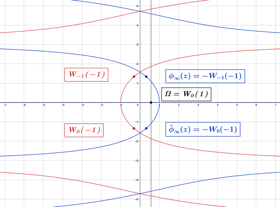
Next, we would like to consider where these numbers sit in the range of the Lambert function. Since is a real constant, it is straightforward to see that it sits on the positive real-axis of the range. It turns out the numeric values of and sit on the branches of Lambert function's range, which we recall were the solutions derived from the expression
(1.2.224)
Figure 1.2.8 – The function's real range around the origin, with positive branches in red
and negative branches in blue, where the following constants lie on the branch cuts:
Figure 1.2.8 represents a plot of the range of the Lambert function centered around the origin, where and are located on the negative real-valued branches, corresponding to the numbers and on positive real-valued branches. These numbers, when taken together, have the following inverse relationships
(1.2.225)
(1.2.226)
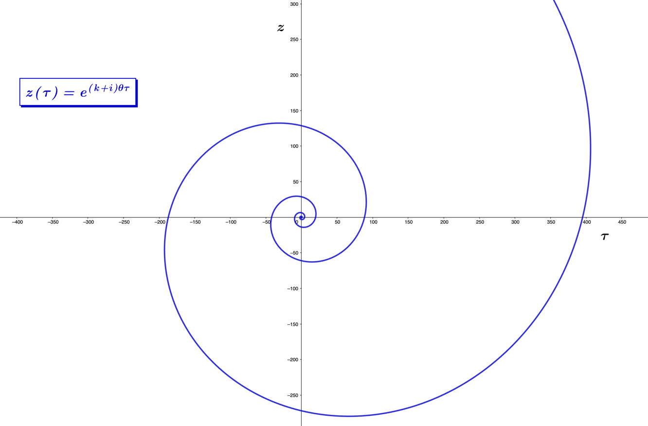
In Figure 1.2.9, we plot the points representing the inverse numbers , which also sit on the real branch cuts in the Lambert function's range. The takeaway from the previous two plots is that the branch cuts represent the convergence points of the infinitely iterated logarithm of numbers and their inverses, and these branch cuts also serve as the convergence point of the logarithm and exponential functions. The expression, is rooted in the logarithm function, and it is not difficult to see that it is a particular form of the logarithmic spiral. For complex numbers, the logarithmic spiral is defined as
(1.2.227)
where represents the distance from the origin in the complex plane, is the angle from the real-axis, and are constants.
Figure 1.2.9 – The function's real range centered at the origin, with positive branches in red and negative branches in blue, with the addition of the inverse constants, which also sit on the branch cuts: .
When , the logarithmic spiral expression defines the complex circle with the radial component We start by setting in the logarithmic spiral expression
(1.2.228)
and given that
(1.2.229)
Taking the exponent portion from the expression above, we can solve to determine the and values
(1.2.230)
(1.2.231)
and then define the logarithmic spiral expression
(1.2.232)
which has the variable values
(1.2.233)
After the addition of an exponent variable , the logarithmic spiral expression becomes
(1.2.234)
which is plotted in Figure 1.2.10, where characteristic logarithmic spirals can be appreciated.
Figure 1.2.10 – The logarithmic spiral , for ,
The Swiss mathematician Jacob Bernoulli (1655-1705) referred to the logarithmic spiral in Latin as the spira mirabilis, which translates to miraculous spiral. Miraculous to him was the self-similarity property that characterizes the logarithmic spiral, where the overall shape of the spiral remains intact with each curve. Based on their mathematical properties, the numbers we have considered in this section are as miraculous as the logarithmic spirals were to Bernoulli.
Initially, we started this section considering the phase shifts of the group velocity, which were dependent on both the tangent space and the subspace which defined the phase space algebra,
(1.2.235)
The tangent space is revealed for , by setting
(1.2.236)
and the phase space algebra by taking the matrix logarithm of
(1.2.237)
The group derivative and Lie algebras considered in matrix representation theory are associated with the Lambert function. This is seen by setting in the group velocity expression , and observing that this is a matrix form of the expression
(1.2.238)
noting the tangent space algebra represents a matrix version of from the expression . The tangent space also has a unique and specific subtangent space, considered by evaluating the derivative of
(1.2.239)
for which we set , finding the smooth paths through the identity characterizing the subtangent space vectors
(1.2.240)
We assign a variable to the subtangent algebra, and define the group as the exponential mapping
(1.2.241)
where is continuous, having a group velocity , found by evaluating its derivative
(1.2.242)
Like the group velocity, can be expressed as the product
(1.2.243)
which, after setting , takes on the Lambert function's associated expression
(1.2.244)
Fittingly, the evaluation of the group velocity for , yields the subtangent space algebra
(1.2.245)
If our starting point is from the perspective of the group velocity, its Lie algebra, is rooted in a dependency on the tangent space group. To find the dynamical state of that yields this Lie algebra, we solve the following component expression for the variable
(1.2.246)
and using this solution, the group velocity is found to equal
(1.2.247)
By changing the -variable to an iterative form , then defining to be the independent variable of the group, the dependency value for can be generalized for any derivative subtangent group as
(1.2.248)
where is the non-variable algebra from the axis entry of the group derivative Lie algebra , and is the non-variable axis entry algebra from the subalgebra group. We apply this generalization to the last example, which started with the expression
(1.2.249)
where, is the variable that coincides with the tangent space. We multiply both sides by
(1.2.250)
then take the logarithm of both sides
(1.2.251)
noting in this case, the derivative axis algebra is equal to
(1.2.252)
and the axis subalgebra is equal to
(1.2.253)
for the variable set as We substitute the and symbolic forms into the expression
(1.2.254)
and solve for
(1.2.255)
which matches our generalized expression. The generalized dependency solutions for non-derivative subalgebras are
(1.2.256)
which can be demonstrated for the tangent space group
(1.2.257)
and the group's dependency for , is
(1.2.258)
For this case, the solution is
(1.2.259)
which leads to the equality
(1.2.260)
We come full circle and back to these intriguing and marvelous numbers to frame them in the context of group theory by defining the Mirabilis Group.
Definition (1.2.261) – The Mirabilis Group is defined by the algebra sets
for, for which, the numbers are based on the product log functions
and characteristic to these numbers, the following identities hold for the,algebras
The Mirabilis Group represents the Lie algebra anchor point located at the crossroads of the logarithm and exponential functions for the -type groups. Our generalized dependency solution also holds for these algebras and groups
(1.2.262)
where can now represent any infinite number of axis entry subalgebras that exist. For our familiar group case
(1.2.263)
its subgroup dependency is rooted in the Lie algebra of the Mirabilis Group, and has a value for , equal to
(1.2.264)
leading to the following identities
(1.2.265)
(1.2.266)
A logarithmic path of descent exists for all numbers, and for those matrix representations not taking on singular values when applying the infinite iterative logarithm function, the path can be defined as follows:
Definition (1.2.267) – The Logarithmic Path of Descentis the unique set of values that compose the set
where each, is defined recursively by the expression
the function,, defines theorder logarithm of the Lie algebra,,
for, with non-singular values, and it is defined that,
To better understand what is, we choose the complex number example and recursively calculate the first ten values of from its logarithmic function descent
(1.2.268)
where the successive values appear to be converging to the value of . Indeed, by , the descent has approached the convergence value of to within sixteen-digit numerical precision, seen by the values
(1.2.269)
Each value holds the key to what the value for is, seen using the example
(1.2.270)
for , where we find that holds
(1.2.271)
The relationship between and is characterized by the following equivalence
(1.2.272)
which is simple to show, given that the product sum is a telescoping one
(1.2.273)
implying the following identity holds
(1.2.274)
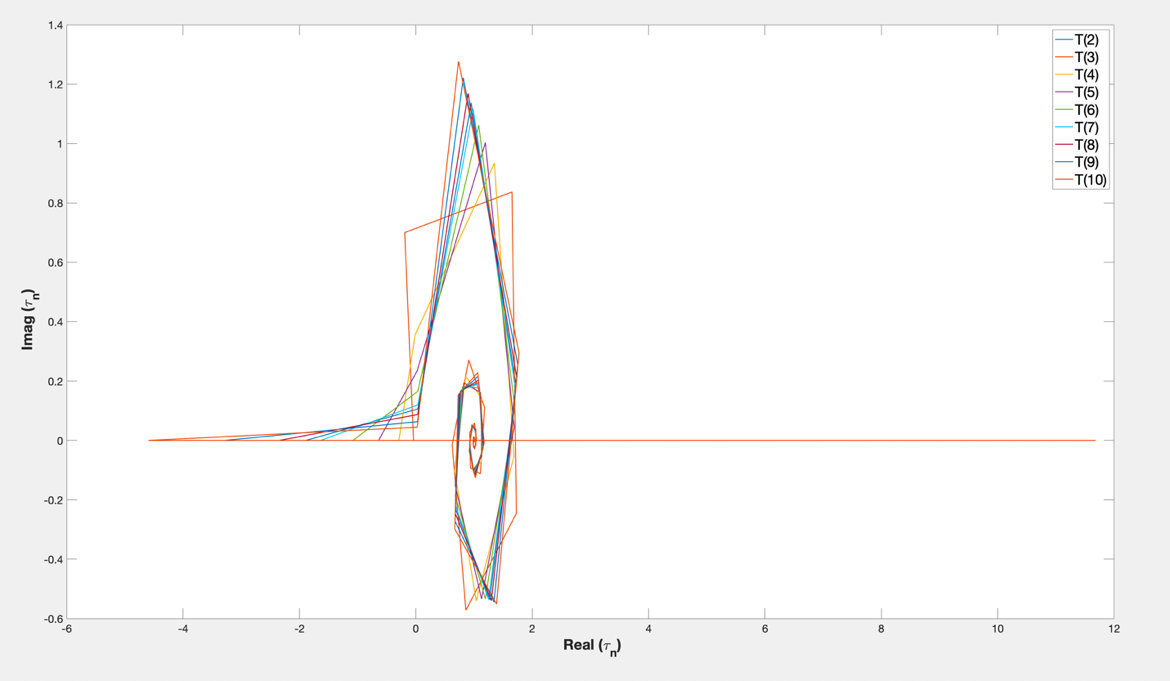
Figure 1.2.11 – Spirals formed by the values for the logarithmic paths of descent, ,of the integers2,
In Figure 1.2.11, we plot the logarithmic paths of descent for the integers two through ten, where a logarithmic-like spiral forms on the descent into the iterations of the logarithm function. Unlike the example of the logarithmic spiral, this is an inward-rotating spiral, where the values of converge to the value of one. The paths of these unique integers are distinct from one another, defining a signature for each number and its informational content. This signature is embodied in the short-hand notation of the variable, where the expression
(1.2.275)
yields the represented number by the product with .
This section's purpose is to highlight the interdependence that exists with all the subspaces composed of unique subalgebras. Each group is connected to its adjacent subgroup through its variable, and that of the subgroup's variable. If an action occurs in one space due to an external influence, the effect is a mathematical propagation of value changes for the variables through the infinite set of algebras that compose its supergroup.