Masteries · Jason GlowneyArithmoí Book 1

Masteries

1.4.4 Null Curves and the Cone Group

As pre­vi­ous­ly dis­cussed, in tra­di­tion­al conic sec­tions, the null curve rep­re­sents lines des­ig­nat­ing the bound­ary of the cone. In the com­plex plane, these lines have slopes taking the form of the pos­i­tive and neg­a­tive square roots of ii, which can be rep­re­sent­ed by the ex­po­nen­tials e(±iπ4),e(±3iπ4)e^{\left( \frac{\pm i\pi}{4} \right)},e^{\left( \frac{\pm 3i\pi}{4} \right)}, and their in­ter­sec­tions with the unit circle. Nu­mer­i­cal­ly, these ex­po­nen­tials rep­re­sent the com­plex num­bers,

(−1)(14)=(12+i2),   (−1)(34)=(−12+i2),( - 1)^{\left( \frac{1}{4} \right)} = \left( \frac{1}{\sqrt{2}} + \frac{i}{\sqrt{2}} \right),\ \ \ ( - 1)^{\left( \frac{3}{4} \right)} = \left( \frac{- 1}{\sqrt{2}} + \frac{i}{\sqrt{2}} \right),
−(−1)(14)=(−12−i2),   −(−1)(34)=(12−i2),\begin{array}{r} {- ( - 1)}^{\left( \frac{1}{4} \right)} = \left( \frac{- 1}{\sqrt{2}} - \frac{i}{\sqrt{2}} \right),\ \ \ {- ( - 1)}^{\left( \frac{3}{4} \right)} = \left( \frac{1}{\sqrt{2}} - \frac{i}{\sqrt{2}} \right), \end{array}
(1.4.60)

with 2×22 \times 2 matrix rep­re­sen­ta­tions

(012+i212+i20),(0−12+i2−12+i20),(0−(12+i2)−(12+i2)0),(012−i212−i20),\begin{array}{r} \begin{pmatrix} 0 & \frac{1}{\sqrt{2}} + \frac{i}{\sqrt{2}} \\ \frac{1}{\sqrt{2}} + \frac{i}{\sqrt{2}} & 0 \end{pmatrix},\begin{pmatrix} 0 & \frac{- 1}{\sqrt{2}} + \frac{i}{\sqrt{2}} \\ \frac{- 1}{\sqrt{2}} + \frac{i}{\sqrt{2}} & 0 \end{pmatrix},\begin{pmatrix} 0 & - \left( \frac{1}{\sqrt{2}} + \frac{i}{\sqrt{2}} \right) \\ - \left( \frac{1}{\sqrt{2}} + \frac{i}{\sqrt{2}} \right) & 0 \end{pmatrix},\begin{pmatrix} 0 & \frac{1}{\sqrt{2}} - \frac{i}{\sqrt{2}} \\ \frac{1}{\sqrt{2}} - \frac{i}{\sqrt{2}} & 0 \end{pmatrix}, \end{array}
(1.4.61)

each of which, squares to

±(i00i).\begin{array}{r} \pm \begin{pmatrix} i & 0 \\ 0 & i \end{pmatrix}. \end{array}
(1.4.62)

There exists a more fun­da­men­tal rep­re­sen­ta­tion of these num­bers, where we argue that these are fun­da­men­tal and anal­o­gous to the imag­i­nary and split com­plex num­bers ∈ℂ2,ℝ2\in \mathbb{C}^{2},\mathbb{R}^{2}

(0ii0),   (0110).\begin{array}{r} \begin{pmatrix} 0 & i \\ i & 0 \end{pmatrix},\ \ \ \begin{pmatrix} 0 & 1 \\ 1 & 0 \end{pmatrix}. \end{array}
(1.4.63)

These num­bers take the forms

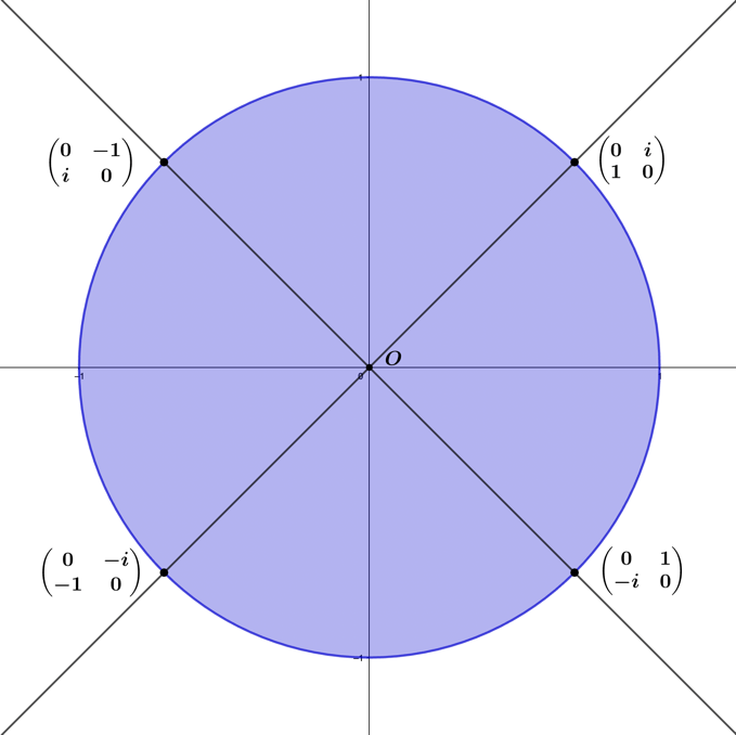
(−1)(14)=(0i10),   (−1)(34)=(0−1i0),( - 1)^{\left( \frac{1}{4} \right)} = \begin{pmatrix} 0 & i \\ 1 & 0 \end{pmatrix},\ \ \ ( - 1)^{\left( \frac{3}{4} \right)} = \begin{pmatrix} 0 & - 1 \\ i & 0 \end{pmatrix},
−(−1)(14)=(0−i−10),   −(−1)(34)=(01−i0),\begin{array}{r} {- ( - 1)}^{\left( \frac{1}{4} \right)} = \begin{pmatrix} 0 & - i \\ - 1 & 0 \end{pmatrix},\ \ \ {- ( - 1)}^{\left( \frac{3}{4} \right)} = \begin{pmatrix} 0 & 1 \\ - i & 0 \end{pmatrix}, \end{array}
(1.4.64)

where ±i,±1\pm i, \pm 1, are arranged on the anti-di­ag­o­nal, having more geo­met­ric sig­nif­i­cance, given that the matrix en­tries al­ter­nate be­tween real and imag­i­nary values. The matrix rep­re­sen­ta­tion for (−1)(14)( - 1)^{\left( \frac{1}{4} \right)}, will square to ii, and when raised to se­quen­tial powers, it will cycle around the unit circle points, (−1)(34),−(−1)(14),−(−1)(34)( - 1)^{\left( \frac{3}{4} \right)},{- ( - 1)}^{\left( \frac{1}{4} \right)},{- ( - 1)}^{\left( \frac{3}{4} \right)}, and the axes of the circle

(0i10)2=(i00i),  (0i10)3=(0−1i0),  (0i10)4=(−100−1),   (0i10)5=(0−i−10),\begin{pmatrix} 0 & i \\ 1 & 0 \end{pmatrix}^{2} = \begin{pmatrix} i & 0 \\ 0 & i \end{pmatrix},\ \ \begin{pmatrix} 0 & i \\ 1 & 0 \end{pmatrix}^{3} = \begin{pmatrix} 0 & - 1 \\ i & 0 \end{pmatrix},\ \ \begin{pmatrix} 0 & i \\ 1 & 0 \end{pmatrix}^{4} = \begin{pmatrix} - 1 & 0 \\ 0 & - 1 \end{pmatrix},\ \ \ \begin{pmatrix} 0 & i \\ 1 & 0 \end{pmatrix}^{5} = \begin{pmatrix} 0 & - i \\ - 1 & 0 \end{pmatrix},
(0i10)6=(−i00−i),   (0i10)7=(01−i0),   (0i10)8=(1001).\begin{array}{r} \begin{pmatrix} 0 & i \\ 1 & 0 \end{pmatrix}^{6} = \begin{pmatrix} - i & 0 \\ 0 & - i \end{pmatrix},\ \ \ \begin{pmatrix} 0 & i \\ 1 & 0 \end{pmatrix}^{7} = \begin{pmatrix} 0 & 1 \\ - i & 0 \end{pmatrix},\ \ \ \begin{pmatrix} 0 & i \\ 1 & 0 \end{pmatrix}^{8} = \begin{pmatrix} 1 & 0 \\ 0 & 1 \end{pmatrix}. \end{array}
(1.4.65)

In Figure 1.4.10, the geom­e­try of the cone num­bers is shown at their in­ter­sec­tion points with the com­plex unit circle.

When com­par­ing the matrix ex­po­nen­tials for the two rep­re­sen­ta­tions of el­e­ments, they differ in the sinh⁡\sinh trigono­met­ric en­tries

exp⁡(0x1(−1)14x1(−1)140)=(cosh⁡(x1(−1)14)sinh⁡(x1(−1)14)sinh⁡(x1(−1)14)cosh⁡(x1(−1)14)),\begin{array}{r} \exp\begin{pmatrix} 0 & x_{1}( - 1)^{\frac{1}{4}} \\ x_{1}( - 1)^{\frac{1}{4}} & 0 \end{pmatrix} = \begin{pmatrix} \cosh\left( x_{1}( - 1)^{\frac{1}{4}} \right) & \sinh\left( x_{1}( - 1)^{\frac{1}{4}} \right) \\ \sinh\left( x_{1}( - 1)^{\frac{1}{4}} \right) & \cosh\left( x_{1}( - 1)^{\frac{1}{4}} \right) \end{pmatrix}, \end{array}
(1.4.66)
exp⁡(0ix1x10)=(cosh⁡(x1(−1)14)(−1)14sinh⁡(x1(−1)14)−(−1)34sinh⁡(x1(−1)14)cosh⁡(x1(−1)14)).\begin{array}{r} \exp\begin{pmatrix} 0 & {ix}_{1} \\ x_{1} & 0 \end{pmatrix} = \begin{pmatrix} \cosh\left( x_{1}( - 1)^{\frac{1}{4}} \right) & {( - 1)^{\frac{1}{4}}\sinh}\left( x_{1}( - 1)^{\frac{1}{4}} \right) \\ {- ( - 1)^{\frac{3}{4}}\sinh}\left( x_{1}( - 1)^{\frac{1}{4}} \right) & \cosh\left( x_{1}( - 1)^{\frac{1}{4}} \right) \end{pmatrix}. \end{array}
(1.4.67)
Figure
Figure 1.4.11 – Cone num­bers on the com­plex unit circle.

Both rep­re­sen­ta­tions are es­sen­tial­ly hy­brids of the trigono­met­ric func­tions of the circle and the hy­per­bo­la, and these can just as easily be rep­re­sent­ed in the forms

exp⁡(0x1(−1)14x1(−1)140)=(cos⁡(−x1(−1)34)isin(−x1(−1)34)isin(−x1(−1)34)cos⁡(−x1(−1)34)),\begin{array}{r} \exp\begin{pmatrix} 0 & x_{1}( - 1)^{\frac{1}{4}} \\ x_{1}( - 1)^{\frac{1}{4}} & 0 \end{pmatrix} = \begin{pmatrix} \cos\left( - x_{1}( - 1)^{\frac{3}{4}} \right) & {isin}\left( - x_{1}( - 1)^{\frac{3}{4}} \right) \\ {isin}\left( - x_{1}( - 1)^{\frac{3}{4}} \right) & \cos\left( - x_{1}( - 1)^{\frac{3}{4}} \right) \end{pmatrix}, \end{array}
(1.4.68)
exp⁡(0ix1x10)=(cos⁡(−x1(−1)34)(−(−1)34) sin(−x1(−1)34)(−(−1)14)sin⁡(−x1(−1)34)cos⁡(−x1(−1)34)).\begin{array}{r} \exp\begin{pmatrix} 0 & ix_{1} \\ x_{1} & 0 \end{pmatrix} = \begin{pmatrix} \cos\left( - x_{1}( - 1)^{\frac{3}{4}} \right) & ({- ( - 1)^{\frac{3}{4}})\ sin}\left( - x_{1}( - 1)^{\frac{3}{4}} \right) \\ {\left( - ( - 1)^{\frac{1}{4}} \right)\sin}\left( - x_{1}( - 1)^{\frac{3}{4}} \right) & \cos\left( - x_{1}( - 1)^{\frac{3}{4}} \right) \end{pmatrix}. \end{array}
(1.4.69)

For matrix de­riv­a­tives, we find­­­­­

ddx1(cosh⁡(x1(−1)14)sinh⁡(x1(−1)14)sinh⁡(x1(−1)14)cosh⁡(x1(−1)14))=((−1)14sinh⁡(x1(−1)14)(−1)14cosh⁡(x1(−1)14)(−1)14cosh⁡(x1(−1)14)(−1)14sinh⁡(x1(−1)14)),\begin{array}{r} \frac{d}{dx_{1}}\begin{pmatrix} \cosh\left( x_{1}( - 1)^{\frac{1}{4}} \right) & \sinh\left( x_{1}( - 1)^{\frac{1}{4}} \right) \\ \sinh\left( x_{1}( - 1)^{\frac{1}{4}} \right) & \cosh\left( x_{1}( - 1)^{\frac{1}{4}} \right) \end{pmatrix} = \begin{pmatrix} ( - 1)^{\frac{1}{4}}\sinh\left( x_{1}( - 1)^{\frac{1}{4}} \right) & ( - 1)^{\frac{1}{4}}\cosh\left( x_{1}( - 1)^{\frac{1}{4}} \right) \\ ( - 1)^{\frac{1}{4}}\cosh\left( x_{1}( - 1)^{\frac{1}{4}} \right) & {( - 1)^{\frac{1}{4}}\sinh}\left( x_{1}( - 1)^{\frac{1}{4}} \right) \end{pmatrix}, \end{array}
(1.4.70)
ddx1(cosh⁡(x1(−1)14)(−1)14sinh⁡(x1(−1)14)−(−1)34sinh⁡(x1(−1)14)cosh⁡(x1(−1)14))=((−1)14sinh⁡(x1(−1)14)icosh(x1(−1)14)cosh⁡(x1(−1)14)(−1)14sinh⁡(x1(−1)14)),\begin{array}{r} \frac{d}{dx_{1}}\begin{pmatrix} \cosh\left( x_{1}( - 1)^{\frac{1}{4}} \right) & {( - 1)^{\frac{1}{4}}\sinh}\left( x_{1}( - 1)^{\frac{1}{4}} \right) \\ {- ( - 1)^{\frac{3}{4}}\sinh}\left( x_{1}( - 1)^{\frac{1}{4}} \right) & \cosh\left( x_{1}( - 1)^{\frac{1}{4}} \right) \end{pmatrix} = \begin{pmatrix} ( - 1)^{\frac{1}{4}}\sinh\left( x_{1}( - 1)^{\frac{1}{4}} \right) & {icosh}\left( x_{1}( - 1)^{\frac{1}{4}} \right) \\ \cosh\left( x_{1}( - 1)^{\frac{1}{4}} \right) & ( - 1)^{\frac{1}{4}}\sinh\left( x_{1}( - 1)^{\frac{1}{4}} \right) \end{pmatrix}, \end{array}
(1.4.71)

re­veal­ing that they will differ by the en­tries on their anti-di­ag­o­nals. When re­lat­ing di­he­dral forms ∈ℂ3\in \mathbb{C}^{3} to the cone num­bers, being con­sid­er­ing, we define the cone number el­e­ments ∈ℂ3\in \mathbb{C}^{3}, by the fol­low­ing,

X1,1=((−1)140000i010),   X2,1=(00i0(−1)140100),   X3,1(0i010000(−1)14),X_{1,1} = \begin{pmatrix} ( - 1)^{\frac{1}{4}} & 0 & 0 \\ 0 & 0 & i \\ 0 & 1 & 0 \end{pmatrix},\ \ \ X_{2,1} = \begin{pmatrix} 0 & 0 & i \\ 0 & ( - 1)^{\frac{1}{4}} & 0 \\ 1 & 0 & 0 \end{pmatrix},\ \ \ X_{3,1}\begin{pmatrix} 0 & i & 0 \\ 1 & 0 & 0 \\ 0 & 0 & ( - 1)^{\frac{1}{4}} \end{pmatrix},
X1,2=((−1)340000−10i0),   X2,2=(00−10(−1)340i00),   X3,2=(0−10i0000(−1)34),X_{1,2} = \begin{pmatrix} ( - 1)^{\frac{3}{4}} & 0 & 0 \\ 0 & 0 & - 1 \\ 0 & i & 0 \end{pmatrix},\ \ \ X_{2,2} = \begin{pmatrix} 0 & 0 & - 1 \\ 0 & ( - 1)^{\frac{3}{4}} & 0 \\ i & 0 & 0 \end{pmatrix},\ \ \ X_{3,2} = \begin{pmatrix} 0 & - 1 & 0 \\ i & 0 & 0 \\ 0 & 0 & ( - 1)^{\frac{3}{4}} \end{pmatrix},
X1,3=(−(−1)140000−i0−10),   X2,3=(00−i0−(−1)340−100),   X3,3=(0−i0−10000−(−1)34),X_{1,3} = \begin{pmatrix} - ( - 1)^{\frac{1}{4}} & 0 & 0 \\ 0 & 0 & - i \\ 0 & - 1 & 0 \end{pmatrix},\ \ \ X_{2,3} = \begin{pmatrix} 0 & 0 & - i \\ 0 & - ( - 1)^{\frac{3}{4}} & 0 \\ - 1 & 0 & 0 \end{pmatrix},\ \ \ X_{3,3} = \begin{pmatrix} 0 & - i & 0 \\ - 1 & 0 & 0 \\ 0 & 0 & {- ( - 1)}^{\frac{3}{4}} \end{pmatrix},
X1,4=(−(−1)34000010−i0),   X2,4=(0010−(−1)140−i00),   X3,4=(010−i0000−(−1)14),\begin{array}{r} X_{1,4} = \begin{pmatrix} - ( - 1)^{\frac{3}{4}} & 0 & 0 \\ 0 & 0 & 1 \\ 0 & - i & 0 \end{pmatrix},\ \ \ X_{2,4} = \begin{pmatrix} 0 & 0 & 1 \\ 0 & {- ( - 1)}^{\frac{1}{4}} & 0 \\ - i & 0 & 0 \end{pmatrix},\ \ \ X_{3,4} = \begin{pmatrix} 0 & 1 & 0 \\ - i & 0 & 0 \\ 0 & 0 & {- ( - 1)}^{\frac{1}{4}} \end{pmatrix}, \end{array}
(1.4.71)

where each el­e­ment is a cone number with re­spec­tive ro­ta­tion­al axes from the set (−1)14,(−1)34,−(−1)14,−(−1)34( - 1)^{\frac{1}{4}},( - 1)^{\frac{3}{4}},{- ( - 1)}^{\frac{1}{4}},{- ( - 1)}^{\frac{3}{4}}. The prod­ucts of these cone num­bers form the el­e­ments of a Cartan al­ge­bra YY of the cone group, a few of which we cal­cu­late prod­ucts with, for Xj,XkX_{j},X_{k}, in­di­cat­ing the set of prod­ucts:

X1,1,X2,k∈{(00(−1)34i000(−1)140),(00−(−1)14−1000(−1)340),(00−(−1)34−i000−(−1)340),(00(−1)141000−(−1)140)},   X1,1,X3,k∈{(0(−1)34000(−1)34100),(0−(−1)14000−(−1)14i00),(0−(−1)14000(−1)14i00),(0−(−1)34000(−1)14−100)},X_{1,1},X_{2,k} \in \left\{ \begin{array}{r} \begin{pmatrix} 0 & 0 & ( - 1)^{\frac{3}{4}} \\ i & 0 & 0 \\ 0 & ( - 1)^{\frac{1}{4}} & 0 \end{pmatrix},\begin{pmatrix} 0 & 0 & {- ( - 1)}^{\frac{1}{4}} \\ - 1 & 0 & 0 \\ 0 & ( - 1)^{\frac{3}{4}} & 0 \end{pmatrix}, \\ \begin{pmatrix} 0 & 0 & - ( - 1)^{\frac{3}{4}} \\ - i & 0 & 0 \\ 0 & {- ( - 1)}^{\frac{3}{4}} & 0 \end{pmatrix},\begin{pmatrix} 0 & 0 & ( - 1)^{\frac{1}{4}} \\ 1 & 0 & 0 \\ 0 & {- ( - 1)}^{\frac{1}{4}} & 0 \end{pmatrix} \end{array} \right\},\ \ \ X_{1,1},X_{3,k} \in \left\{ \begin{array}{r} \begin{pmatrix} 0 & ( - 1)^{\frac{3}{4}} & 0 \\ 0 & 0 & ( - 1)^{\frac{3}{4}} \\ 1 & 0 & 0 \end{pmatrix},\begin{pmatrix} 0 & {- ( - 1)}^{\frac{1}{4}} & 0 \\ 0 & 0 & {- ( - 1)}^{\frac{1}{4}} \\ i & 0 & 0 \end{pmatrix}, \\ \begin{pmatrix} 0 & {- ( - 1)}^{\frac{1}{4}} & 0 \\ 0 & 0 & ( - 1)^{\frac{1}{4}} \\ i & 0 & 0 \end{pmatrix},\begin{pmatrix} 0 & {- ( - 1)}^{\frac{3}{4}} & 0 \\ 0 & 0 & ( - 1)^{\frac{1}{4}} \\ - 1 & 0 & 0 \end{pmatrix} \end{array} \right\},
X2,1,X3,k∈{(00(−1)34(−1)14000i0),(00−(−1)14(−1)34000−10),(00(−1)14−(−1)34000−i0),(00−(−1)34−(−1)3400010)},   X2,1,X1,k∈{(0i000(−1)34(−1)1400),(0−1000−(−1)14(−1)3400),(0−i000−(−1)34−(−1)1400),(01000(−1)14−(−1)3400)},X_{2,1},X_{3,k} \in \left\{ \begin{array}{r} \begin{pmatrix} 0 & 0 & ( - 1)^{\frac{3}{4}} \\ ( - 1)^{\frac{1}{4}} & 0 & 0 \\ 0 & i & 0 \end{pmatrix},\begin{pmatrix} 0 & 0 & {- ( - 1)}^{\frac{1}{4}} \\ ( - 1)^{\frac{3}{4}} & 0 & 0 \\ 0 & - 1 & 0 \end{pmatrix}, \\ \begin{pmatrix} 0 & 0 & ( - 1)^{\frac{1}{4}} \\ {- ( - 1)}^{\frac{3}{4}} & 0 & 0 \\ 0 & - i & 0 \end{pmatrix},\begin{pmatrix} 0 & 0 & {- ( - 1)}^{\frac{3}{4}} \\ {- ( - 1)}^{\frac{3}{4}} & 0 & 0 \\ 0 & 1 & 0 \end{pmatrix} \end{array} \right\},\ \ \ X_{2,1},X_{1,k} \in \left\{ \begin{array}{r} \begin{pmatrix} 0 & i & 0 \\ 0 & 0 & ( - 1)^{\frac{3}{4}} \\ ( - 1)^{\frac{1}{4}} & 0 & 0 \end{pmatrix},\begin{pmatrix} 0 & - 1 & 0 \\ 0 & 0 & {- ( - 1)}^{\frac{1}{4}} \\ ( - 1)^{\frac{3}{4}} & 0 & 0 \end{pmatrix}, \\ \begin{pmatrix} 0 & - i & 0 \\ 0 & 0 & - ( - 1)^{\frac{3}{4}} \\ {- ( - 1)}^{\frac{1}{4}} & 0 & 0 \end{pmatrix},\begin{pmatrix} 0 & 1 & 0 \\ 0 & 0 & ( - 1)^{\frac{1}{4}} \\ {- ( - 1)}^{\frac{3}{4}} & 0 & 0 \end{pmatrix} \end{array} \right\},
X3,1,X2,k∈{(0(−1)34000i(−1)1400),(0−(−1)14000−1(−1)3400),(0(−1)14000−i−(−1)1400),(0(−1)340001−(−1)3400)},   X3,1,X1,k∈{(00−1(−1)14000(−1)140),(00−i(−1)34000(−1)340),(001−(−1)14000−(−1)140),(00i−(−1)34000−(−1)340)}.\begin{array}{r} X_{3,1},X_{2,k} \in \left\{ \begin{array}{r} \begin{pmatrix} 0 & ( - 1)^{\frac{3}{4}} & 0 \\ 0 & 0 & i \\ ( - 1)^{\frac{1}{4}} & 0 & 0 \end{pmatrix},\begin{pmatrix} 0 & {- ( - 1)}^{\frac{1}{4}} & 0 \\ 0 & 0 & - 1 \\ ( - 1)^{\frac{3}{4}} & 0 & 0 \end{pmatrix}, \\ \begin{pmatrix} 0 & ( - 1)^{\frac{1}{4}} & 0 \\ 0 & 0 & - i \\ {- ( - 1)}^{\frac{1}{4}} & 0 & 0 \end{pmatrix},\begin{pmatrix} 0 & ( - 1)^{\frac{3}{4}} & 0 \\ 0 & 0 & 1 \\ {- ( - 1)}^{\frac{3}{4}} & 0 & 0 \end{pmatrix} \end{array} \right\},\ \ \ X_{3,1},X_{1,k} \in \left\{ \begin{array}{r} \begin{pmatrix} 0 & 0 & - 1 \\ ( - 1)^{\frac{1}{4}} & 0 & 0 \\ 0 & ( - 1)^{\frac{1}{4}} & 0 \end{pmatrix},\begin{pmatrix} 0 & 0 & - i \\ ( - 1)^{\frac{3}{4}} & 0 & 0 \\ 0 & ( - 1)^{\frac{3}{4}} & 0 \end{pmatrix}, \\ \begin{pmatrix} 0 & 0 & 1 \\ - ( - 1)^{\frac{1}{4}} & 0 & 0 \\ 0 & {- ( - 1)}^{\frac{1}{4}} & 0 \end{pmatrix},\begin{pmatrix} 0 & 0 & i \\ {- ( - 1)}^{\frac{3}{4}} & 0 & 0 \\ 0 & - ( - 1)^{\frac{3}{4}} & 0 \end{pmatrix} \end{array} \right\}. \end{array}
(1.4.72)

The Xj,XkX_{j},X_{k} prod­uct re­sults are sim­i­lar in form to the Y2,Y3Y_{2},Y_{3} Cartan sub­al­ge­bras from the other di­he­dral groups

Y2=(0a000bc00),   Y3=(00ab000c0),\begin{array}{r} Y_{2} = \begin{pmatrix} 0 & a & 0 \\ 0 & 0 & b \\ c & 0 & 0 \end{pmatrix},\ \ \ Y_{3} = \begin{pmatrix} 0 & 0 & a \\ b & 0 & 0 \\ 0 & c & 0 \end{pmatrix}, \end{array}
(1.4.73)

and for the Y1Y_{1} el­e­ments

Y1=(a000b000c).\begin{array}{r} Y_{1} = \begin{pmatrix} a & 0 & 0 \\ 0 & b & 0 \\ 0 & 0 & c \end{pmatrix}. \end{array}
(1.4.74)

In the case of a Y1Y_{1} per­mu­ta­tion matrix, for which, a,b,c=1a,b,c = 1, we have the mul­ti­plica­tive iden­ti­ty ϵ\epsilon of the group. The sim­plest means for a cone number el­e­ment to trans­form to the iden­ti­ty ϵ\epsilon, is by suc­ces­sive self-prod­ucts

X1,18=((−1)140000i010)8=(100010001)=ϵ.\begin{array}{r} X_{1,1}^{8} = \begin{pmatrix} ( - 1)^{\frac{1}{4}} & 0 & 0 \\ 0 & 0 & i \\ 0 & 1 & 0 \end{pmatrix}^{8} = \begin{pmatrix} 1 & 0 & 0 \\ 0 & 1 & 0 \\ 0 & 0 & 1 \end{pmatrix} = \epsilon. \end{array}
(1.4.75)

For entry values {a,b,c}\{ a,b,c\}, sim­i­lar rep­re­sen­ta­tions in­clu­sive of all XjX_{j}-type per­mu­ta­tions, take the gen­er­al form

Xj={(a0000b0c0),   (00b0a0c00),   (0b0c0000a)}.\begin{array}{r} X_{j} = \left\{ \begin{pmatrix} a & 0 & 0 \\ 0 & 0 & b \\ 0 & c & 0 \end{pmatrix},\ \ \ \begin{pmatrix} 0 & 0 & b \\ 0 & a & 0 \\ c & 0 & 0 \end{pmatrix},\ \ \ \begin{pmatrix} 0 & b & 0 \\ c & 0 & 0 \\ 0 & 0 & a \end{pmatrix} \right\}. \end{array}
(1.4.76)

The group being con­sid­er­ing is com­prised of a much larger set of per­mu­ta­tion el­e­ments in com­par­i­son to the other di­he­dral groups cov­ered up to this point. The values for each entry a,b,ca,b,c can be any com­plex number from the set of eight el­e­ments {1,(−1)(14),i,(−1)(34),−1,−(−1)(14),−i,−(−1)(34)}.\left\{ 1,( - 1)^{\left( \frac{1}{4} \right)},i,( - 1)^{\left( \frac{3}{4} \right)}, - 1,{- ( - 1)}^{\left( \frac{1}{4} \right)}, - i,{- ( - 1)}^{\left( \frac{3}{4} \right)} \right\}.The XjX_{j} el­e­ments are a sub­group of the larger D3𝕔D_{3\mathbb{c}} group, where for in­stance, we can derive X1,1∈D3𝕔X_{1,1} \in D_{3\mathbb{c}}, by way of the fol­low­ing com­bi­na­tion of prod­ucts (X3,1X2,1X3,1X1,16)\left( X_{3,1}X_{2,1}X_{3,1}X_{1,1}^{6} \right)

((0i010000(−1)14)(00i0(−1)140100)(0i010000(−1)14)((−1)140000i010)6)=((−1)140000(−1)140(−1)140).\begin{array}{r} \left( \begin{pmatrix} 0 & i & 0 \\ 1 & 0 & 0 \\ 0 & 0 & ( - 1)^{\frac{1}{4}} \end{pmatrix}\begin{pmatrix} 0 & 0 & i \\ 0 & ( - 1)^{\frac{1}{4}} & 0 \\ 1 & 0 & 0 \end{pmatrix}\begin{pmatrix} 0 & i & 0 \\ 1 & 0 & 0 \\ 0 & 0 & ( - 1)^{\frac{1}{4}} \end{pmatrix}\begin{pmatrix} ( - 1)^{\frac{1}{4}} & 0 & 0 \\ 0 & 0 & i \\ 0 & 1 & 0 \end{pmatrix}^{6} \right) = \begin{pmatrix} ( - 1)^{\frac{1}{4}} & 0 & 0 \\ 0 & 0 & ( - 1)^{\frac{1}{4}} \\ 0 & ( - 1)^{\frac{1}{4}} & 0 \end{pmatrix}. \end{array}
(1.4.77)

In like fash­ion, the re­main­ing two el­e­ments X2,1,X3,1∈D3𝕔X_{2,1},X_{3,1} \in D_{3\mathbb{c}}, can be gen­er­at­ed by the fol­low­ing prod­ucts

X2,1∈D3𝕔=(X1,1X3,1,X1,17)=(00(−1)140(−1)140(−1)1400),\begin{array}{r} X_{2,1} \in D_{3\mathbb{c}} = \left( X_{1,1}X_{3,1},X_{1,1}^{7} \right) = \begin{pmatrix} 0 & 0 & ( - 1)^{\frac{1}{4}} \\ 0 & ( - 1)^{\frac{1}{4}} & 0 \\ ( - 1)^{\frac{1}{4}} & 0 & 0 \end{pmatrix}, \end{array}
(1.4.78)
X3,1∈D3𝕔=(X2,1X1,1,X2,17)=(0(−1)140(−1)140000(−1)14).\begin{array}{r} X_{3,1} \in D_{3\mathbb{c}} = \left( X_{2,1}X_{1,1},X_{2,1}^{7} \right) = \begin{pmatrix} 0 & ( - 1)^{\frac{1}{4}} & 0 \\ ( - 1)^{\frac{1}{4}} & 0 & 0 \\ 0 & 0 & ( - 1)^{\frac{1}{4}} \end{pmatrix}. \end{array}
(1.4.79)

The fa­mil­iar Cartan sub­al­ge­bra forms Yj,Y_{j},can be gen­er­at­ed by the prod­ucts X2,1X3,1n,X1,1X2,1X2,1X1,1{X_{2,1}X_{3,1}^{n},X_{1,1}X}_{2,1}X_{2,1}X_{1,1}, for n=1,3,5,7n = 1,3,5,7,

( n=1)=(0−i000−i−i00),   ( n=3)=(010001100),(\ n = 1) = \begin{pmatrix} 0 & - i & 0 \\ 0 & 0 & - i \\ - i & 0 & 0 \end{pmatrix},\ \ \ (\ n = 3) = \begin{pmatrix} 0 & 1 & 0 \\ 0 & 0 & 1 \\ 1 & 0 & 0 \end{pmatrix},
( n=5)=(0i000ii00),   ( n=7)=(0−1000−1−100).\begin{array}{r} (\ n = 5) = \begin{pmatrix} 0 & i & 0 \\ 0 & 0 & i \\ i & 0 & 0 \end{pmatrix},\ \ \ (\ n = 7) = \begin{pmatrix} 0 & - 1 & 0 \\ 0 & 0 & - 1 \\ - 1 & 0 & 0 \end{pmatrix}. \end{array}
(1.4.80)

Con­cern­ing cone number per­mu­ta­tion ma­tri­ces of the YjY_{j}-type*,* they are not nec­es­sar­i­ly com­mu­ta­tive as they were for the Cartan sub­al­ge­bras from pre­vi­ous stud­ies. This is be­cause the per­mu­ta­tion ma­tri­ces ∈Yj\in Y_{j} can now vary in their in­di­vid­ual entry values, which are drawn from the set {1,(−1)(14),i,(−1)(34),−1,−(−1)(14),−i,−(−1)(34)}.\left\{ 1,( - 1)^{\left( \frac{1}{4} \right)},i,( - 1)^{\left( \frac{3}{4} \right)}, - 1,{- ( - 1)}^{\left( \frac{1}{4} \right)}, - i,{- ( - 1)}^{\left( \frac{3}{4} \right)} \right\}.For the Y2,Y3Y_{2},Y_{3}-type ma­tri­ces, a cyclic shift in the entry values occurs for the Lie brack­et op­er­a­tion

(0a000bc00)(00de000f0)=(ae000bf000cd)≠(00de000f0)(0a000bc00)=(cd000ae000bf).\begin{array}{r} \begin{pmatrix} 0 & a & 0 \\ 0 & 0 & b \\ c & 0 & 0 \end{pmatrix}\begin{pmatrix} 0 & 0 & d \\ e & 0 & 0 \\ 0 & f & 0 \end{pmatrix} = \begin{pmatrix} ae & 0 & 0 \\ 0 & bf & 0 \\ 0 & 0 & cd \end{pmatrix} \neq \begin{pmatrix} 0 & 0 & d \\ e & 0 & 0 \\ 0 & f & 0 \end{pmatrix}\begin{pmatrix} 0 & a & 0 \\ 0 & 0 & b \\ c & 0 & 0 \end{pmatrix} = \begin{pmatrix} cd & 0 & 0 \\ 0 & ae & 0 \\ 0 & 0 & bf \end{pmatrix}. \end{array}
(1.4.81)

More suc­cinct­ly, we can de­scribe the com­mu­ta­tor re­la­tion­ships, as

[Y2,Y3]=(ae−cd000bf−ae000cd−bf),\begin{array}{r} \left\lbrack Y_{2},Y_{3} \right\rbrack = \begin{pmatrix} ae - cd & 0 & 0 \\ 0 & bf - ae & 0 \\ 0 & 0 & cd - bf \end{pmatrix}, \end{array}
(1.4.82)
[Y3,Y2]=(cd−ae000ae−bf000bf−cd),\begin{array}{r} \left\lbrack Y_{3},Y_{2} \right\rbrack = \begin{pmatrix} cd - ae & 0 & 0 \\ 0 & ae - bf & 0 \\ 0 & 0 & bf - cd \end{pmatrix}, \end{array}
(1.4.83)

which im­plies that for the Y2,Y3Y_{2},Y_{3} ma­tri­ces to com­mute, we must have that ae=cd=bfae = cd = bf.

By these con­sid­er­a­tions, we can now define the cone group ∈ℂ3\in \mathbb{C}^{3}, as fol­lows:

De­f­i­n­i­tion (1.4.84) – The di­he­dral cone group 𝐃𝟑ℂ𝚫\mathbf{D}_{\mathbf{3}\mathbb{C}}^{\boldsymbol{\Delta}}, is de­fined as a group under com­po­si­tion that sits in the com­plex geo­met­ric space ℂ3×3\mathbb{C}^{3 \times 3}, with a set AΔA^{\Delta} of per­mu­ta­tion el­e­ments, with the su­per­script Δ,\Delta, rep­re­sent­ing the cone.

AΔ ={AΔ∈U(3,ℂ)|AΔ∙AΔ†=I }.\begin{array}{r} A^{\Delta}\ = \left\{ A^{\Delta} \in U\left( 3,\mathbb{C} \right)|A^{\Delta} \bullet {A^{\Delta}}^{\dagger} = I\ \right\}. \end{array}

The­o­rem (1.4.85) – The set of per­mu­ta­tions AΔA^{\Delta} forms a group under com­po­si­tion

Proof – Ver­i­fi­ca­tion of group axioms

  • Clo­sure: All el­e­ments ∈AΔ\in A^{\Delta} are bi­jec­tive, and the com­po­si­tion of any el­e­ments ϕ∘ψ ∈AΔ\phi \circ \psi\ \in A^{\Delta} is also bi­jec­tive.
  • As­so­cia­tiv­i­ty: Per­mu­ta­tions are func­tions, and their com­po­si­tions are as­so­cia­tive.
  • Iden­ti­ty: The iden­ti­ty func­tion ϵ AΔ\epsilon_{\ A^{\Delta}} bi­jec­tive­ly maps all el­e­ments of the set AΔA^{\Delta} to them­selves (ϵAΔ:AΔ→AΔ)\left( \epsilon_{A^{\Delta}}:A^{\Delta} \rightarrow A^{\Delta} \right).
  • In­verse: ϕ\phi is a per­mu­ta­tion and is thus bi­jec­tive, and there exists a func­tion ϕ−1\phi^{- 1} that is also bi­jec­tive.
□\square

The­o­rem (1.4.86) – The di­he­dral cone group D3ℂΔD_{3\mathbb{C}}^{\Delta} con­tains a total of 1,536 per­mu­ta­tion el­e­ments ∈ℂ3\in \mathbb{C}^{3}, where el­e­ments of Xj∈𝒳X_{j}\in \mathcal{X} are each com­prised of 256 per­mu­ta­tions with cone num­bers for their de­ter­mi­nants, and the el­e­ments Yj∈𝒴Y_{j}\in \mathcal{Y} are also each com­prised of 256 el­e­ments with axis num­bers for their de­ter­mi­nants.

𝐏𝐫𝐨𝐨𝐟−\mathbf{Proof}\mathbf{-} ∀ Xj,k\forall\ X_{j,k} el­e­ments, de­ter­mi­nants are com­plex num­bers on the unit circle, lo­cat­ed on cone points from the set {1,(−1)(14),i,(−1)(34),−1,−(−1)(14),−i,−(−1)(34)}\left\{ 1,( - 1)^{\left( \frac{1}{4} \right)},i,( - 1)^{\left( \frac{3}{4} \right)}, - 1,{- ( - 1)}^{\left( \frac{1}{4} \right)}, - i,{- ( - 1)}^{\left( \frac{3}{4} \right)} \right\}, and specif­i­cal­ly, the el­e­ments ∈Xj,1\in X_{j,1} have de­ter­mi­nants equal to −(−1)(34)- ( - 1)^{\left( \frac{3}{4} \right)}. For el­e­ments ∈Yj,k\in Y_{j,k}, they also have com­plex number de­ter­mi­nants on the unit circle, lo­cat­ed at axis points from the set {1,−i,−1,i}\left\{ 1, - i, - 1,i \right\}, and specif­i­cal­ly, the el­e­ments ∈Yj,1\in Y_{j,1} have de­ter­mi­nants equal to −i- i . From linear al­ge­bra, the prod­uct of de­ter­mi­nants is equal to de­ter­mi­nant of the matrix-matrix prod­uct

det⁡(AB)=det⁡(A)×det⁡(B),\det(AB) = \det(A) \times \det(B),

and the fol­low­ing prod­uct re­la­tions for the D3D_{3} di­he­dral groups, hold con­gru­ent modulo 3,

Xj2=Y1,  XjXj+1=Y3,  XjXj−1=Y2,  XjY2=Xj−1,  XjY3=Xj+1,X_{j}^{2} = Y_{1},\ \ X_{j}X_{j + 1} = Y_{3},\ \ X_{j}X_{j - 1} = Y_{2},\ \ X_{j}Y_{2} = X_{j - 1},\ \ X_{j}Y_{3} = X_{j + 1},
Y2Xj=Xj+1,  Y3Xj=Xj−1,  Y2Y3=Y1,  Y22=Y3,  Y32=Y2.Y_{2}X_{j} = X_{j + 1},\ \ Y_{3}X_{j} = X_{j - 1},\ \ Y_{2}Y_{3} = Y_{1},\ \ Y_{2}^{2} = Y_{3},\ \ Y_{3}^{2} = Y_{2}.

From these prod­uct re­la­tion­ships of group el­e­ments and de­ter­mi­nants, the 𝒴\mathcal{Y}-el­e­ment de­ter­mi­nants will always remain on the axes of the unit circle, and the 𝒳\mathcal{X}-el­e­ment de­ter­mi­nants will always be cone number points on unit circle. Fur­ther, the prod­uct re­sults of any even powers in­volv­ing 𝒳\mathcal{X}, will always be on the axes and ∈\in 𝒴\mathcal{Y}, for ex­am­ple

X1,j4X2,k8∈𝒴.X_{1,j}^{4}X_{2,k}^{8}\in \mathcal{Y}.

The sum of two even ex­po­nents yield an even ex­po­nent result and based on the prod­uct re­la­tion­ship 𝒳j𝒳k∈𝒴\mathcal{X}_{j}\mathcal{X}_{k}\in \mathcal{Y}, any prod­uct com­bi­na­tion of el­e­ments ∈𝒳\in \mathcal{X} that re­sults in an even ex­po­nent is always ∈𝒴\in \mathcal{Y}. All odd power ex­po­nent sums of el­e­ment prod­uct of com­bi­na­tions ∈𝒳\in \mathcal{X}, result in a cone number de­ter­mi­nant matrix, based on the unit circle's sym­me­try and the el­e­ment prod­uct re­la­tion­ships, which are always ∈𝒳\in \mathcal{X}. For ex­am­ple,

X1,j3X2,k6∈𝒳,X_{1,j}^{3}X_{2,k}^{6}\in \mathcal{X},

has an odd num­bered sum for the prod­uct ex­po­nents 3+6=93 + 6 = 9, and always holds, since any even+odd=oddeven + odd = odd. This is the case for the re­sults of prod­ucts ∈𝒳\in \mathcal{X}, and not prod­ucts ∈𝒴\in \mathcal{Y}, and/or the com­bi­na­tion of prod­ucts ∈𝒳,𝒴.\in \mathcal{X},\mathcal{Y}. The reason is the fol­low­ing de­ter­mi­nant holds, det⁡(XjmXkn)=det⁡(Xjm)×det⁡(Xkn)\det\left( X_{j}^{m}X_{k}^{n} \right) = \det\left( X_{j}^{m} \right) \times \det\left( X_{k}^{n} \right). This im­plies that for m,n=odd,evenm,n = odd,even and/or even/odd, the result is a matrix de­ter­mi­nant that is a cone number and there­fore ∈𝒳\in \mathcal{X}. While any com­bi­na­tions, m,n=odd,odd,n = odd,odd and/or even/even result in an axis num­bered matrix de­ter­mi­nant, and is there­fore, ∈𝒴\in \mathcal{Y}. The de­ter­mi­nants are cal­cu­lat­ed by the prod­ucts of the three en­tries in each el­e­ment ∈𝒳,𝒴\in \mathcal{X},\mathcal{Y}. For cone num­bered de­ter­mi­nants, these en­tries must have values that are an arrange­ment of ACCACC or CAACAA, where CC, de­fines a cone number, and AA, an axis number. For ex­am­ple, the X1,1X_{1,1}matrix has CAACAA for its en­tries, and its de­ter­mi­nant is

det⁡((−1)14(C)0000i(A)01(A)0)=(−1)14(C)×det(0i(A)1(A)0)=(−1)14∙−i(CAA)=−(−134),\det\begin{pmatrix} ( - 1)^{\frac{1}{4}}(C) & 0 & 0 \\ 0 & 0 & i(A) \\ 0 & 1(A) & 0 \end{pmatrix} = ( - 1)^{\frac{1}{4}}(C) \times det\begin{pmatrix} 0 & i(A) \\ 1(A) & 0 \end{pmatrix} = ( - 1)^{\frac{1}{4}} \bullet - i(CAA) = - \left( - 1^{\frac{3}{4}} \right),

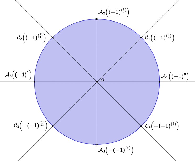
where the prod­uct CAACAA, gives a cone number result. When taking the de­ter­mi­nant prod­uct of ma­tri­ces ∈D3ℂΔ\in D_{3\mathbb{C}}^{\Delta}, this re­la­tion­ship will always hold and de­ter­mines if the result is ∈𝒳\in \mathcal{X}, for cone num­bers, and ∈𝒴\in \mathcal{Y}, for axis num­bers. For clar­i­fi­ca­tion of these num­bers, we see in Figure 1.4.12 the arrange­ment of cone num­bers and axis num­bers on the unit circle and their sym­me­try.

Figure
Figure 1.4.12 – Cone num­bers CC and axis num­bers AA, on the com­plex unit circle.

For all ma­tri­ces Xj,k∈𝒳X_{j,k}\in \mathcal{X}, the arrange­ment of cone num­bers and axis num­bers can be one of four pos­si­ble forms for each Xj,kX_{j,k}:

{(C0000A0A0),(C0000C0C0),(A0000C0A0),(A0000A0C0)}∈X1,k,\left\{ \begin{pmatrix} C & 0 & 0 \\ 0 & 0 & A \\ 0 & A & 0 \end{pmatrix},\begin{pmatrix} C & 0 & 0 \\ 0 & 0 & C \\ 0 & C & 0 \end{pmatrix},\begin{pmatrix} A & 0 & 0 \\ 0 & 0 & C \\ 0 & A & 0 \end{pmatrix},\begin{pmatrix} A & 0 & 0 \\ 0 & 0 & A \\ 0 & C & 0 \end{pmatrix} \right\} \in X_{1,k},
{(00A0C0A00),(00C0C0C00),(00C0A0A00),(00A0A0C00)}∈X2,k,\left\{ \begin{pmatrix} 0 & 0 & A \\ 0 & C & 0 \\ A & 0 & 0 \end{pmatrix},\begin{pmatrix} 0 & 0 & C \\ 0 & C & 0 \\ C & 0 & 0 \end{pmatrix},\begin{pmatrix} 0 & 0 & C \\ 0 & A & 0 \\ A & 0 & 0 \end{pmatrix},\begin{pmatrix} 0 & 0 & A \\ 0 & A & 0 \\ C & 0 & 0 \end{pmatrix} \right\} \in X_{2,k},
{(0A0A0000C),(0C0C0000C),(0C0A0000A),(0A0C0000A)}∈X3,k.\left\{ \begin{pmatrix} 0 & A & 0 \\ A & 0 & 0 \\ 0 & 0 & C \end{pmatrix},\begin{pmatrix} 0 & C & 0 \\ C & 0 & 0 \\ 0 & 0 & C \end{pmatrix},\begin{pmatrix} 0 & C & 0 \\ A & 0 & 0 \\ 0 & 0 & A \end{pmatrix},\begin{pmatrix} 0 & A & 0 \\ C & 0 & 0 \\ 0 & 0 & A \end{pmatrix} \right\} \in X_{3,k}.

And for the ma­tri­ces with el­e­ments ∈𝒴\in \mathcal{Y}, each Yj,kY_{j,k} form will also have four pos­si­ble forms:

{(A000A000A),(C000C000A),(A000C000C),(C000A000C)}∈Y1,k,\left\{ \begin{pmatrix} A & 0 & 0 \\ 0 & A & 0 \\ 0 & 0 & A \end{pmatrix},\begin{pmatrix} C & 0 & 0 \\ 0 & C & 0 \\ 0 & 0 & A \end{pmatrix},\begin{pmatrix} A & 0 & 0 \\ 0 & C & 0 \\ 0 & 0 & C \end{pmatrix},\begin{pmatrix} C & 0 & 0 \\ 0 & A & 0 \\ 0 & 0 & C \end{pmatrix} \right\} \in Y_{1,k},
{(0A000AA00),(0C000CA00),(0A000CC00),(0C000AC00)}∈Y2,k,\left\{ \begin{pmatrix} 0 & A & 0 \\ 0 & 0 & A \\ A & 0 & 0 \end{pmatrix},\begin{pmatrix} 0 & C & 0 \\ 0 & 0 & C \\ A & 0 & 0 \end{pmatrix},\begin{pmatrix} 0 & A & 0 \\ 0 & 0 & C \\ C & 0 & 0 \end{pmatrix},\begin{pmatrix} 0 & C & 0 \\ 0 & 0 & A \\ C & 0 & 0 \end{pmatrix} \right\} \in Y_{2,k},
{(00AA000A0),(00AC000C0),(00CA000C0),(00CC000A0)}∈Y3,k.\left\{ \begin{pmatrix} 0 & 0 & A \\ A & 0 & 0 \\ 0 & A & 0 \end{pmatrix},\begin{pmatrix} 0 & 0 & A \\ C & 0 & 0 \\ 0 & C & 0 \end{pmatrix},\begin{pmatrix} 0 & 0 & C \\ A & 0 & 0 \\ 0 & C & 0 \end{pmatrix},\begin{pmatrix} 0 & 0 & C \\ C & 0 & 0 \\ 0 & A & 0 \end{pmatrix} \right\} \in Y_{3,k}.

As there are four dif­fer­ent num­bers in each group A{1,i,−1,−i},  C{(−1)14,(−1)34,−(−1)14,−(−1)34}A\left\{ 1,i, - 1, - i \right\},\ \ C\left\{ ( - 1)^{\frac{1}{4}},( - 1)^{\frac{3}{4}}, - ( - 1)^{\frac{1}{4}}, - ( - 1)^{\frac{3}{4}} \right\}, there are 43=644^{3} = 64 pos­si­ble per­mu­ta­tions for each matrix above, and given there are a total of 24 matrix forms above, there are 64×24=153664 \times 24 = 1536 el­e­ments total in the group.

The brute force por­tion of this proof now fol­lows. Since we must show that all these per­mu­ta­tion pos­si­bil­i­ties are indeed achiev­able by mul­ti­plica­tive clo­sure of the el­e­ments X1,1,X2,1,X3,1X_{1,1},X_{2,1},X_{3,1}. We start by defin­ing per­mu­ta­tion el­e­ments (Mj=1,2,3n)\left( M_{j = 1,2,3}^{n} \right) in the form of  Y1,k\ Y_{1,k} ma­tri­ces with main di­ag­o­nals en­tries

((X3,15X2,1X3,1X1,15)2X3,1X2,1X3,1X1,15)n=(1000−(−1)14000(−1)34)n=M1n,\left( \left( X_{3,1}^{5}X_{2,1}X_{3,1}X_{1,1}^{5} \right)^{2}X_{3,1}X_{2,1}X_{3,1}X_{1,1}^{5} \right)^{n} = \begin{pmatrix} 1 & 0 & 0 \\ 0 & {- ( - 1)}^{\frac{1}{4}} & 0 \\ 0 & 0 & ( - 1)^{\frac{3}{4}} \end{pmatrix}^{n} = M_{1}^{n},
((X2,1(X3,1X1,1)2)2)n=(1000(−1)34000(−1)34)n=M2n,\left( \left( X_{2,1}\left( X_{3,1}X_{1,1} \right)^{2} \right)^{2} \right)^{n} = \begin{pmatrix} 1 & 0 & 0 \\ 0 & ( - 1)^{\frac{3}{4}} & 0 \\ 0 & 0 & ( - 1)^{\frac{3}{4}} \end{pmatrix}^{n} = M_{2}^{n},
(X3,1X2,1X3,1X1,15)n=(1000−(−1)34000(−1)14)n=M3n,\left( X_{3,1}X_{2,1}X_{3,1}X_{1,1}^{5} \right)^{n} = \begin{pmatrix} 1 & 0 & 0 \\ 0 & {- ( - 1)}^{\frac{3}{4}} & 0 \\ 0 & 0 & ( - 1)^{\frac{1}{4}} \end{pmatrix}^{n} = M_{3}^{n},

and fur­ther define the matrix el­e­ment Y2=M4nY_{2} = M_{4}^{n}, as

X2,1X3,13,X2,1X1,1X2,1X1,1=(010001100)=M4n.{X_{2,1}X_{3,1}^{3},X_{2,1}X}_{1,1}X_{2,1}X_{1,1} = \begin{pmatrix} 0 & 1 & 0 \\ 0 & 0 & 1 \\ 1 & 0 & 0 \end{pmatrix} = M_{4}^{n}.

We start by work­ing on the X1,kX_{1,k}-per­mu­ta­tions for the number arrange­ments

(C0000C0C0),   (C0000A0A0),\begin{pmatrix} C & 0 & 0 \\ 0 & 0 & C \\ 0 & C & 0 \end{pmatrix},\ \ \ \begin{pmatrix} C & 0 & 0 \\ 0 & 0 & A \\ 0 & A & 0 \end{pmatrix},

while taking X1,1X_{1,1}, as

X1,1=((−1)140000i010).X_{1,1} = \begin{pmatrix} ( - 1)^{\frac{1}{4}} & 0 & 0 \\ 0 & 0 & i \\ 0 & 1 & 0 \end{pmatrix}.

Since all MjnM_{j}^{n} have el­e­ment a1,1=1a_{1,1} = 1, all prod­ucts MjnX1,1M_{j}^{n}X_{1,1} will yield the same value (−1)14 ,( - 1)^{\frac{1}{4}}\ , for a1,1a_{1,1} in the X1,kX_{1,k}-matrix result. To save space, we dis­play the re­sults of these prod­uct trans­for­ma­tions in a 3×13 \times 1 vector no­ta­tion,

MX=(a1,10000a2,30a3,20)→(a1,1a2,3a3,2).MX = \begin{pmatrix} a_{1,1} & 0 & 0 \\ 0 & 0 & a_{2,3} \\ 0 & a_{3,2} & 0 \end{pmatrix} \rightarrow \begin{pmatrix} a_{1,1} \\ a_{2,3} \\ a_{3,2} \end{pmatrix}.

For the forms, (C0000C0C0)\begin{pmatrix} C & 0 & 0 \\ 0 & 0 & C \\ 0 & C & 0 \end{pmatrix}, we pro­ceed to find the six­teen com­bi­na­tions for our fixed cone number, C, at a1,1a_{1,1}, using the fol­low­ing prod­ucts

M1nX1,1=((−1)14−(−1)34(−1)34)n=1,((−1)14(−1)14(−1)14)n=3,((−1)14(−1)34−(−1)34)n=5,((−1)14−(−1)14−(−1)14)n=7,M_{1}^{n}X_{1,1} = \begin{pmatrix} ( - 1)^{\frac{1}{4}} \\ {- ( - 1)}^{\frac{3}{4}} \\ ( - 1)^{\frac{3}{4}} \end{pmatrix}_{n = 1},\begin{pmatrix} ( - 1)^{\frac{1}{4}} \\ ( - 1)^{\frac{1}{4}} \\ ( - 1)^{\frac{1}{4}} \end{pmatrix}_{n = 3},\begin{pmatrix} ( - 1)^{\frac{1}{4}} \\ ( - 1)^{\frac{3}{4}} \\ {- ( - 1)}^{\frac{3}{4}} \end{pmatrix}_{n = 5},\begin{pmatrix} ( - 1)^{\frac{1}{4}} \\ {- ( - 1)}^{\frac{1}{4}} \\ {- ( - 1)}^{\frac{1}{4}} \end{pmatrix}_{n = 7},
M2nX1,1=((−1)14−(−1)14(−1)34)n=1,((−1)14(−1)34(−1)14)n=3,((−1)14(−1)14−(−1)34)n=5,((−1)14−(−1)34−(−1)14)n=7,M_{2}^{n}X_{1,1} = \begin{pmatrix} ( - 1)^{\frac{1}{4}} \\ {- ( - 1)}^{\frac{1}{4}} \\ ( - 1)^{\frac{3}{4}} \end{pmatrix}_{n = 1},\begin{pmatrix} ( - 1)^{\frac{1}{4}} \\ ( - 1)^{\frac{3}{4}} \\ ( - 1)^{\frac{1}{4}} \end{pmatrix}_{n = 3},\begin{pmatrix} ( - 1)^{\frac{1}{4}} \\ ( - 1)^{\frac{1}{4}} \\ {- ( - 1)}^{\frac{3}{4}} \end{pmatrix}_{n = 5},\begin{pmatrix} ( - 1)^{\frac{1}{4}} \\ - ( - 1)^{\frac{3}{4}} \\ {- ( - 1)}^{\frac{1}{4}} \end{pmatrix}_{n = 7},
M3nX1,1=((−1)14(−1)14(−1)14)n=1,((−1)14−(−1)34(−1)34)n=3,((−1)14−(−1)14−(−1)14)n=5,((−1)14(−1)34−(−1)34)n=7,M_{3}^{n}X_{1,1} = \begin{pmatrix} ( - 1)^{\frac{1}{4}} \\ ( - 1)^{\frac{1}{4}} \\ ( - 1)^{\frac{1}{4}} \end{pmatrix}_{n = 1},\begin{pmatrix} ( - 1)^{\frac{1}{4}} \\ {- ( - 1)}^{\frac{3}{4}} \\ ( - 1)^{\frac{3}{4}} \end{pmatrix}_{n = 3},\begin{pmatrix} ( - 1)^{\frac{1}{4}} \\ - ( - 1)^{\frac{1}{4}} \\ {- ( - 1)}^{\frac{1}{4}} \end{pmatrix}_{n = 5},\begin{pmatrix} ( - 1)^{\frac{1}{4}} \\ ( - 1)^{\frac{3}{4}} \\ {- ( - 1)}^{\frac{3}{4}} \end{pmatrix}_{n = 7},
(M1M22)nX1,1=((−1)14−(−1)14(−1)14)n=1,((−1)14(−1)34(−1)34)n=3,((−1)14(−1)14−(−1)14)n=5,((−1)14−(−1)34−(−1)34)n=7.\left( {M_{1}M}_{2}^{2} \right)^{n}X_{1,1} = \begin{pmatrix} ( - 1)^{\frac{1}{4}} \\ {- ( - 1)}^{\frac{1}{4}} \\ ( - 1)^{\frac{1}{4}} \end{pmatrix}_{n = 1},\begin{pmatrix} ( - 1)^{\frac{1}{4}} \\ ( - 1)^{\frac{3}{4}} \\ ( - 1)^{\frac{3}{4}} \end{pmatrix}_{n = 3},\begin{pmatrix} ( - 1)^{\frac{1}{4}} \\ ( - 1)^{\frac{1}{4}} \\ {- ( - 1)}^{\frac{1}{4}} \end{pmatrix}_{n = 5},\begin{pmatrix} ( - 1)^{\frac{1}{4}} \\ - ( - 1)^{\frac{3}{4}} \\ {- ( - 1)}^{\frac{3}{4}} \end{pmatrix}_{n = 7}.

For the forms, (C0000A0A0)\begin{pmatrix} C & 0 & 0 \\ 0 & 0 & A \\ 0 & A & 0 \end{pmatrix}, the re­main­ing six­teen per­mu­ta­tion com­bi­na­tions for CC at a1,1a_{1,1}, we use the fol­low­ing prod­ucts

(M1M2)nX1,1=((−1)14i−i)n=1,((−1)14i−1)n=2,((−1)14ii)n=3,\left( {M_{1}M}_{2} \right)^{n}X_{1,1} = \begin{pmatrix} ( - 1)^{\frac{1}{4}} \\ i \\ - i \end{pmatrix}_{n = 1},\begin{pmatrix} ( - 1)^{\frac{1}{4}} \\ i \\ - 1 \end{pmatrix}_{n = 2},\begin{pmatrix} ( - 1)^{\frac{1}{4}} \\ i \\ i \end{pmatrix}_{n = 3},
(M1M23)nX1,1=((−1)141−1)n=1,((−1)14−i1)n=2,((−1)14−1−1)n=3,\left( {M_{1}M}_{2}^{3} \right)^{n}X_{1,1} = \begin{pmatrix} ( - 1)^{\frac{1}{4}} \\ 1 \\ - 1 \end{pmatrix}_{n = 1},\begin{pmatrix} ( - 1)^{\frac{1}{4}} \\ - i \\ 1 \end{pmatrix}_{n = 2},\begin{pmatrix} ( - 1)^{\frac{1}{4}} \\ - 1 \\ - 1 \end{pmatrix}_{n = 3},
(M12M22)nX1,1=((−1)14i−1)n=1,((−1)14i1)n=2,\left( {M_{1}^{2}M}_{2}^{2} \right)^{n}X_{1,1} = \begin{pmatrix} ( - 1)^{\frac{1}{4}} \\ i \\ - 1 \end{pmatrix}_{n = 1},\begin{pmatrix} ( - 1)^{\frac{1}{4}} \\ i \\ 1 \end{pmatrix}_{n = 2},
(M12M24)nX1,1=((−1)141i)n=1,((−1)14−i−1)n=2,((−1)14−1−i)n=3,\left( {M_{1}^{2}M}_{2}^{4} \right)^{n}X_{1,1} = \begin{pmatrix} ( - 1)^{\frac{1}{4}} \\ 1 \\ i \end{pmatrix}_{n = 1},\begin{pmatrix} ( - 1)^{\frac{1}{4}} \\ - i \\ - 1 \end{pmatrix}_{n = 2},\begin{pmatrix} ( - 1)^{\frac{1}{4}} \\ - 1 \\ - i \end{pmatrix}_{n = 3},
(M15M2)nX1,1=((−1)14−ii)n=1,((−1)14−i−i)n=3,\left( {M_{1}^{5}M}_{2} \right)^{n}X_{1,1} = \begin{pmatrix} ( - 1)^{\frac{1}{4}} \\ - i \\ i \end{pmatrix}_{n = 1},\begin{pmatrix} ( - 1)^{\frac{1}{4}} \\ - i \\ - i \end{pmatrix}_{n = 3},
(M17M2)nX1,1=((−1)1411)n=1,((−1)14−11)n=3.\left( {M_{1}^{7}M}_{2} \right)^{n}X_{1,1} = \begin{pmatrix} ( - 1)^{\frac{1}{4}} \\ 1 \\ 1 \end{pmatrix}_{n = 1},\begin{pmatrix} ( - 1)^{\frac{1}{4}} \\ - 1 \\ 1 \end{pmatrix}_{n = 3}.

In total there are fif­teen dis­tinct per­mu­ta­tions above, where X1,1X_{1,1} has the same form, (C0000A0A0)\begin{pmatrix} C & 0 & 0 \\ 0 & 0 & A \\ 0 & A & 0 \end{pmatrix}, and the six­teenth group per­mu­ta­tion is simply our orig­i­nal X1,1X_{1,1} el­e­ment

X1,1=((−1)14i1).X_{1,1 =}\begin{pmatrix} ( - 1)^{\frac{1}{4}} \\ i \\ 1 \end{pmatrix}.

To find the re­main­ing X1,kX_{1,k} per­mu­ta­tions, re­quires find­ing all forms of the 32 ma­tri­ces above, having a cone number for its a1,1a_{1,1}-el­e­ment. To do so, we need to iden­ti­fy the fol­low­ing per­mu­ta­tions ma­tri­ces,

X1,k=((−1)340000i010),   (−(−1)140000i010),   (−(−1)340000i010),X_{1,k} = \begin{pmatrix} ( - 1)^{\frac{3}{4}} & 0 & 0 \\ 0 & 0 & i \\ 0 & 1 & 0 \end{pmatrix},\ \ \ \begin{pmatrix} {- ( - 1)}^{\frac{1}{4}} & 0 & 0 \\ 0 & 0 & i \\ 0 & 1 & 0 \end{pmatrix},\ \ \ \begin{pmatrix} {- ( - 1)}^{\frac{3}{4}} & 0 & 0 \\ 0 & 0 & i \\ 0 & 1 & 0 \end{pmatrix},

having the same 2×22 \times 2 bottom-right sub­ma­trix as the X1,1X_{1,1}-per­mu­ta­tions, and then simply apply all the same trans­for­ma­tions pre­vi­ous­ly done for the X1,1X_{1,1} matrix. Find­ing per­mu­ta­tion prod­ucts to yield these ma­tri­ces re­quires a map­ping X1,(2,3,4)→X1,kX_{1,(2,3,4)} \rightarrow X_{1,k}, de­not­ed in the bold font in the fol­low­ing ma­tri­ces,

((−1)340000−10i0)(𝟏𝟎𝟎𝟎−𝐢𝟎𝟎𝟎−𝐢)=((−1)340000i010),\begin{pmatrix} ( - 1)^{\frac{3}{4}} & 0 & 0 \\ 0 & 0 & - 1 \\ 0 & i & 0 \end{pmatrix}\begin{pmatrix} \mathbf{1} & \mathbf{0} & \mathbf{0} \\ \mathbf{0} & - \mathbf{i} & \mathbf{0} \\ \mathbf{0} & \mathbf{0} & - \mathbf{i} \end{pmatrix} = \begin{pmatrix} ( - 1)^{\frac{3}{4}} & 0 & 0 \\ 0 & 0 & i \\ 0 & 1 & 0 \end{pmatrix},
(−(−1)140000−i0−10)(𝟏𝟎𝟎𝟎−𝟏𝟎𝟎𝟎−𝟏)=(−(−1)140000i010),\begin{pmatrix} - ( - 1)^{\frac{1}{4}} & 0 & 0 \\ 0 & 0 & - i \\ 0 & - 1 & 0 \end{pmatrix}\begin{pmatrix} \mathbf{1} & \mathbf{0} & \mathbf{0} \\ \mathbf{0} & - \mathbf{1} & \mathbf{0} \\ \mathbf{0} & \mathbf{0} & - \mathbf{1} \end{pmatrix}\mathbf{=}\begin{pmatrix} {- ( - 1)}^{\frac{1}{4}} & 0 & 0 \\ 0 & 0 & i \\ 0 & 1 & 0 \end{pmatrix},
(−(−1)34000010−i0)(𝟏𝟎𝟎𝟎𝐢𝟎𝟎𝟎𝐢)=(−(−1)340000i010).\begin{pmatrix} {- ( - 1)}^{\frac{3}{4}} & 0 & 0 \\ 0 & 0 & 1 \\ 0 & - i & 0 \end{pmatrix}\begin{pmatrix} \mathbf{1} & \mathbf{0} & \mathbf{0} \\ \mathbf{0} & \mathbf{i} & \mathbf{0} \\ \mathbf{0} & \mathbf{0} & \mathbf{i} \end{pmatrix}\mathbf{=}\begin{pmatrix} {- ( - 1)}^{\frac{3}{4}} & 0 & 0 \\ 0 & 0 & i \\ 0 & 1 & 0 \end{pmatrix}.

By using the prod­uct com­bi­na­tions of our pre­vi­ous ma­tri­ces M1mM2n{M_{1}^{m}M}_{2}^{n}, we find so­lu­tions for these map­ping ma­tri­ces

M18M22=(1000−i000−i),   M14M28=(1000−1000−1), M14M22=(1000i000i),{M_{1}^{8}M}_{2}^{2} = \begin{pmatrix} 1 & 0 & 0 \\ 0 & - i & 0 \\ 0 & 0 & - i \end{pmatrix},\ \ \ {M_{1}^{4}M}_{2}^{8} = \begin{pmatrix} 1 & 0 & 0 \\ 0 & - 1 & 0 \\ 0 & 0 & - 1 \end{pmatrix},{{\ M}_{1}^{4}M}_{2}^{2} = \begin{pmatrix} 1 & 0 & 0 \\ 0 & i & 0 \\ 0 & 0 & i \end{pmatrix},

and after ap­ply­ing the same map­pings for the first 32 per­mu­ta­tions, this brings us to a total of 128 per­mu­ta­tions for the X1,kX_{1,k} el­e­ments.

The other X1,kX_{1,k}-el­e­ment per­mu­ta­tions, come by con­sid­er­ing the second half of the matrix number forms

(A0000C0A0),   (A0000A0C0),\begin{pmatrix} A & 0 & 0 \\ 0 & 0 & C \\ 0 & A & 0 \end{pmatrix},\ \ \ \begin{pmatrix} A & 0 & 0 \\ 0 & 0 & A \\ 0 & C & 0 \end{pmatrix},

for a1,1a_{1,1}, an axis number, and the two en­tries in the 2×22 \times 2 bottom-right sub­ma­trix will al­ter­nate be­tween axis and cone num­bers. To arrive at the form above, the en­tries of the left matrix must be mapped by the row/column trans­for­ma­tions: a3,2→a1,1,  a1,1→a2,3,  a2,3→a3,2a_{3,2} \rightarrow a_{1,1},\ \ a_{1,1} \rightarrow a_{2,3},\ \ a_{2,3} \rightarrow a_{3,2}, and onto the right matrix. For the matrix X1,1X_{1,1}, this map­ping rep­re­sents

X1,1→X1,1′=(a1,10000a2,30a3,20)→(a3,20000a1,10a2,30)=((−1)140000i010)→(10000(−1)140i0).X_{1,1} \rightarrow X_{1,1}^{'} = \begin{pmatrix} a_{1,1} & 0 & 0 \\ 0 & 0 & a_{2,3} \\ 0 & a_{3,2} & 0 \end{pmatrix} \rightarrow \begin{pmatrix} a_{3,2} & 0 & 0 \\ 0 & 0 & a_{1,1} \\ 0 & a_{2,3} & 0 \end{pmatrix} = \begin{pmatrix} ( - 1)^{\frac{1}{4}} & 0 & 0 \\ 0 & 0 & i \\ 0 & 1 & 0 \end{pmatrix} \rightarrow \begin{pmatrix} 1 & 0 & 0 \\ 0 & 0 & ( - 1)^{\frac{1}{4}} \\ 0 & i & 0 \end{pmatrix}.

To ac­com­plish this, we use the fol­low­ing matrix prod­ucts

X1,1′=(X2,1X3,1X1,15X2,1X3,1)=(10000(−1)140i0).X_{1,1}^{'} = \left( X_{2,1}X_{3,1}X_{1,1}^{5}X_{2,1}X_{3,1} \right) = \begin{pmatrix} 1 & 0 & 0 \\ 0 & 0 & ( - 1)^{\frac{1}{4}} \\ 0 & i & 0 \end{pmatrix}.

To de­ter­mine the X1,1′X_{1,1}^{'} trans­for­ma­tions, we pro­ceed by ap­ply­ing the same X1,1X_{1,1} trans­for­ma­tions to find six­teen el­e­ments of the form

(10000A0C0),\begin{pmatrix} 1 & 0 & 0 \\ 0 & 0 & A \\ 0 & C & 0 \end{pmatrix},

by way of the fol­low­ing prod­ucts:

M1nX′1,1=(1−i−(−1)14)n=1,(11(−1)34)n=3,(1i(−1)14)n=5,(1−1−(−1)34)n=7,M_{1}^{n}{X'}_{1,1} = \begin{pmatrix} 1 \\ - i \\ {- ( - 1)}^{\frac{1}{4}} \end{pmatrix}_{n = 1}{,\begin{pmatrix} 1 \\ 1 \\ ( - 1)^{\frac{3}{4}} \end{pmatrix}}_{n = 3},\begin{pmatrix} 1 \\ i \\ ( - 1)^{\frac{1}{4}} \end{pmatrix}_{n = 5},\begin{pmatrix} 1 \\ - 1 \\ {- ( - 1)}^{\frac{3}{4}} \end{pmatrix}_{n = 7},
M2nX′1,1=(1−1−(−1)14)n=1,(1i(−1)34)n=3,(11(−1)14)n=5,(1−i−(−1)34)n=7,M_{2}^{n}{X'}_{1,1} = \begin{pmatrix} 1 \\ - 1 \\ {- ( - 1)}^{\frac{1}{4}} \end{pmatrix}_{n = 1}{,\begin{pmatrix} 1 \\ i \\ ( - 1)^{\frac{3}{4}} \end{pmatrix}}_{n = 3},\begin{pmatrix} 1 \\ 1 \\ ( - 1)^{\frac{1}{4}} \end{pmatrix}_{n = 5},\begin{pmatrix} 1 \\ - i \\ {- ( - 1)}^{\frac{3}{4}} \end{pmatrix}_{n = 7},
(M2M12)nX′1,1=(1−i(−1)34)n=1,(11−(−1)14)n=3,(1i−(−1)34)n=5,(1−1(−1)14)n=7,\left( {M_{2}M}_{1}^{2} \right)^{n}{X'}_{1,1} = \begin{pmatrix} 1 \\ - i \\ ( - 1)^{\frac{3}{4}} \end{pmatrix}_{n = 1}{,\begin{pmatrix} 1 \\ 1 \\ {- ( - 1)}^{\frac{1}{4}} \end{pmatrix}}_{n = 3},\begin{pmatrix} 1 \\ i \\ {- ( - 1)}^{\frac{3}{4}} \end{pmatrix}_{n = 5},\begin{pmatrix} 1 \\ - 1 \\ ( - 1)^{\frac{1}{4}} \end{pmatrix}_{n = 7},
(M1M22)nX′1,1=(1−1(−1)34)n=1,(1i−(−1)14)n=3,(11−(−1)34)n=5,(1−i(−1)14)n=7.\left( {M_{1}M}_{2}^{2} \right)^{n}{X'}_{1,1} = \begin{pmatrix} 1 \\ - 1 \\ ( - 1)^{\frac{3}{4}} \end{pmatrix}_{n = 1}{,\begin{pmatrix} 1 \\ i \\ {- ( - 1)}^{\frac{1}{4}} \end{pmatrix}}_{n = 3},\begin{pmatrix} 1 \\ 1 \\ {- ( - 1)}^{\frac{3}{4}} \end{pmatrix}_{n = 5},\begin{pmatrix} 1 \\ - i \\ ( - 1)^{\frac{1}{4}} \end{pmatrix}_{n = 7}.

The re­main­ing six­teen el­e­ments of the form

(10000C0A0),\begin{pmatrix} 1 & 0 & 0 \\ 0 & 0 & C \\ 0 & A & 0 \end{pmatrix},

are then found by the closed mul­ti­pli­ca­tion trans­for­ma­tions:

(M1M2)nX′1,1=(1(−1)141)n=1,(1(−1)14−i)n=2,(1(−1)14−1)n=3,\left( {M_{1}M}_{2} \right)^{n}{X'}_{1,1} = \begin{pmatrix} 1 \\ ( - 1)^{\frac{1}{4}} \\ 1 \end{pmatrix}_{n = 1},\begin{pmatrix} 1 \\ ( - 1)^{\frac{1}{4}} \\ - i \end{pmatrix}_{n = 2},\begin{pmatrix} 1 \\ ( - 1)^{\frac{1}{4}} \\ - 1 \end{pmatrix}_{n = 3},
(M1M23)nX′1,1=(1−(−1)34−i)n=1,(1−(−1)14i)n=2,(1(−1)34−i)n=3,\left( {M_{1}M}_{2}^{3} \right)^{n}{X'}_{1,1} = \begin{pmatrix} 1 \\ {- ( - 1)}^{\frac{3}{4}} \\ - i \end{pmatrix}_{n = 1},\begin{pmatrix} 1 \\ {- ( - 1)}^{\frac{1}{4}} \\ i \end{pmatrix}_{n = 2},\begin{pmatrix} 1 \\ ( - 1)^{\frac{3}{4}} \\ - i \end{pmatrix}_{n = 3},
(M14M22)nX′1,1=(1(−1)34−1)n=1,(1−(−1)341)n=3,\left( {M_{1}^{4}M}_{2}^{2} \right)^{n}{X'}_{1,1} = \begin{pmatrix} 1 \\ ( - 1)^{\frac{3}{4}} \\ - 1 \end{pmatrix}_{n = 1},\begin{pmatrix} 1 \\ {- ( - 1)}^{\frac{3}{4}} \\ 1 \end{pmatrix}_{n = 3},
(M12M24)nX′1,1=(1−(−1)34−1)n=1,(1−(−1)14−i)n=2,(1(−1)341)n=3,\left( {M_{1}^{2}M}_{2}^{4} \right)^{n}{X'}_{1,1} = \begin{pmatrix} 1 \\ {- ( - 1)}^{\frac{3}{4}} \\ - 1 \end{pmatrix}_{n = 1},\begin{pmatrix} 1 \\ {- ( - 1)}^{\frac{1}{4}} \\ - i \end{pmatrix}_{n = 2},\begin{pmatrix} 1 \\ ( - 1)^{\frac{3}{4}} \\ 1 \end{pmatrix}_{n = 3},
(M15M2)nX′1,1=(1−(−1)14−1)n=1,(1−(−1)141)n=3,\left( {M_{1}^{5}M}_{2} \right)^{n}{X'}_{1,1} = \begin{pmatrix} 1 \\ {- ( - 1)}^{\frac{1}{4}} \\ - 1 \end{pmatrix}_{n = 1},\begin{pmatrix} 1 \\ {- ( - 1)}^{\frac{1}{4}} \\ 1 \end{pmatrix}_{n = 3},
(M17M2)nX′1,1=(1−(−1)34i)n=1,(1(−1)34i)n=3,\left( {M_{1}^{7}M}_{2} \right)^{n}{X'}_{1,1} = \begin{pmatrix} 1 \\ {- ( - 1)}^{\frac{3}{4}} \\ i \end{pmatrix}_{n = 1},\begin{pmatrix} 1 \\ ( - 1)^{\frac{3}{4}} \\ i \end{pmatrix}_{n = 3},

which com­prise fif­teen dif­fer­ent per­mu­ta­tions, and the six­teenth is simply our X1,1′X_{1,1}^{'} matrix

X′1,1=(1(−1)14i).{X'}_{1,1 =}\begin{pmatrix} 1 \\ ( - 1)^{\frac{1}{4}} \\ i \end{pmatrix}.

To arrive at the re­main­ing per­mu­ta­tions of X′1{X'}_{1}, it re­quires iden­ti­fy­ing the fol­low­ing per­mu­ta­tions

X1,k′=(i0000(−1)140i0),   (−10000(−1)140i0),   (−i0000(−1)140i0),X_{1,k}^{'} = \begin{pmatrix} i & 0 & 0 \\ 0 & 0 & ( - 1)^{\frac{1}{4}} \\ 0 & i & 0 \end{pmatrix},\ \ \ \begin{pmatrix} - 1 & 0 & 0 \\ 0 & 0 & ( - 1)^{\frac{1}{4}} \\ 0 & i & 0 \end{pmatrix},\ \ \ \begin{pmatrix} - i & 0 & 0 \\ 0 & 0 & ( - 1)^{\frac{1}{4}} \\ 0 & i & 0 \end{pmatrix},

having a 2×22 \times 2 bottom-right sub­ma­trix equal to that found in the X′1,1{X'}_{1,1}per­mu­ta­tion. We then we apply the same X′1,1{X'}_{1,1} trans­for­ma­tions, giving us the fol­low­ing ma­tri­ces de­not­ed in bold below, which map X′1,1→X1,k′{X'}_{1,1} \rightarrow X_{1,k}^{'}:

(𝐢𝟎𝟎𝟎𝟏𝟎𝟎𝟎𝟏)(10000(−1)140i0)=(i0000(−1)140i0),\begin{pmatrix} \mathbf{i} & \mathbf{0} & \mathbf{0} \\ \mathbf{0} & \mathbf{1} & \mathbf{0} \\ \mathbf{0} & \mathbf{0} & \mathbf{1} \end{pmatrix}\begin{pmatrix} 1 & 0 & 0 \\ 0 & 0 & ( - 1)^{\frac{1}{4}} \\ 0 & i & 0 \end{pmatrix} = \begin{pmatrix} i & 0 & 0 \\ 0 & 0 & ( - 1)^{\frac{1}{4}} \\ 0 & i & 0 \end{pmatrix},
(−𝟏𝟎𝟎𝟎−(−𝟏)𝟏𝟒𝟎𝟎𝟎−(−𝟏)𝟏𝟒)(10000−10−(−1)140)=(−10000(−1)140i0),\begin{pmatrix} - \mathbf{1} & \mathbf{0} & \mathbf{0} \\ \mathbf{0} & \mathbf{-}\left( - \mathbf{1} \right)^{\frac{\mathbf{1}}{\mathbf{4}}} & \mathbf{0} \\ \mathbf{0} & \mathbf{0} & \mathbf{-}\left( - \mathbf{1} \right)^{\frac{\mathbf{1}}{\mathbf{4}}} \end{pmatrix}\begin{pmatrix} 1 & 0 & 0 \\ 0 & 0 & - 1 \\ 0 & {- ( - 1)}^{\frac{1}{4}} & 0 \end{pmatrix}\mathbf{=}\begin{pmatrix} - 1 & 0 & 0 \\ 0 & 0 & ( - 1)^{\frac{1}{4}} \\ 0 & i & 0 \end{pmatrix},
(−𝐢𝟎𝟎𝟎i𝟎𝟎𝟎i)(10000−(−1)34010)=(−i0000(−1)140i0).\begin{pmatrix} - \mathbf{i} & \mathbf{0} & \mathbf{0} \\ \mathbf{0} & i & \mathbf{0} \\ \mathbf{0} & \mathbf{0} & i \end{pmatrix}\begin{pmatrix} 1 & 0 & 0 \\ 0 & 0 & {- ( - 1)}^{\frac{3}{4}} \\ 0 & 1 & 0 \end{pmatrix}\mathbf{=}\begin{pmatrix} - i & 0 & 0 \\ 0 & 0 & ( - 1)^{\frac{1}{4}} \\ 0 & i & 0 \end{pmatrix}.

By using the prod­uct com­bi­na­tions M2nM_{2}^{n}, XjnX_{j}^{n}, so­lu­tions are found by eval­u­at­ing the prod­ucts

X1,12M22=(i00010001),   (X1,12M22)2(X3,1X1,1X2,1)2=(−1000−(−1)14000−(−1)14),   X1,16M24=(−i000i000i).X_{1,1}^{2}M_{2}^{2} = \begin{pmatrix} i & 0 & 0 \\ 0 & 1 & 0 \\ 0 & 0 & 1 \end{pmatrix}\mathbf{,\ \ \ }{\left( X_{1,1}^{2}M_{2}^{2} \right)^{2}\left( X_{3,1}X_{1,1}X_{2,1} \right)}^{2} = \begin{pmatrix} - 1 & 0 & 0 \\ 0 & - ( - 1)^{\frac{1}{4}} & 0 \\ 0 & 0 & - ( - 1)^{\frac{1}{4}} \end{pmatrix},\ \ \ X_{1,1}^{6}M_{2}^{4} = \begin{pmatrix} - i & 0 & 0 \\ 0 & i & 0 \\ 0 & 0 & i \end{pmatrix}\mathbf{.}

With com­plete so­lu­tions for all cone group per­mu­ta­tions X1,k,X′1,j∈𝒳1X_{1,k},{X'}_{1,j} \in \mathcal{X}_{1}, we find the values for all re­main­ing X2,X′2,X3,X3′X_{2},{X'}_{2,}X_{3},X_{3}^{'}, per­mu­ta­tions by using the Cartan sub­al­ge­bra el­e­ment Y3Y_{3}, found by using the prod­uct trans­for­ma­tion

M41=(001100010).M_{4}^{1} = \begin{pmatrix} 0 & 0 & 1 \\ 1 & 0 & 0 \\ 0 & 1 & 0 \end{pmatrix}.

So, the fol­low­ing trans­for­ma­tions yield 𝒳2,𝒳3\mathcal{X}_{2},\mathcal{X}_{3}, as fol­lows

𝒳1(001100010)=𝒳2,  (001100010)𝒳1=𝒳3.\mathcal{X}_{1}\begin{pmatrix} 0 & 0 & 1 \\ 1 & 0 & 0 \\ 0 & 1 & 0 \end{pmatrix} = \mathcal{X}_{2},\ \ \begin{pmatrix} 0 & 0 & 1 \\ 1 & 0 & 0 \\ 0 & 1 & 0 \end{pmatrix}\mathcal{X}_{1} = \mathcal{X}_{3}.

All per­mu­ta­tions in 𝒳\mathcal{X} have now been found, to­tal­ing 64×4×3=76864 \times 4 \times 3 = 768 per­mu­ta­tions. Fi­nal­ly, to prove that we have all the per­mu­ta­tion el­e­ments ∈𝒴1,𝒴2,𝒴3\in \mathcal{Y}_{1},\mathcal{Y}_{2},\mathcal{Y}_{3}, we recall that

(X3,1X2,1X3,1X1,16)=((−1)140000(−1)140(−1)140),\left( X_{3,1}X_{2,1}X_{3,1}X_{1,1}^{6} \right) = \begin{pmatrix} ( - 1)^{\frac{1}{4}} & 0 & 0 \\ 0 & 0 & ( - 1)^{\frac{1}{4}} \\ 0 & ( - 1)^{\frac{1}{4}} & 0 \end{pmatrix},

which when acting on an­oth­er per­mu­ta­tion ∈𝒳\in \mathcal{X} , will result in a per­mu­ta­tion matrix ∈𝒴\in \mathcal{Y}, having uni­form­ly ro­tat­ed el­e­ments by (−1)(14)( - 1)^{\left( \frac{1}{4} \right)} . Ap­ply­ing this linear trans­for­ma­tion to the 𝒳\mathcal{X} per­mu­ta­tion el­e­ments, yields the 𝒴1,𝒴2,𝒴3\mathcal{Y}_{1},\mathcal{Y}_{2},\mathcal{Y}_{3}, el­e­ments

X1,k((−1)140000(−1)140(−1)140)=Y1,k,X_{1,k}\begin{pmatrix} ( - 1)^{\frac{1}{4}} & 0 & 0 \\ 0 & 0 & ( - 1)^{\frac{1}{4}} \\ 0 & ( - 1)^{\frac{1}{4}} & 0 \end{pmatrix} = Y_{1,k},
X2,k((−1)140000(−1)140(−1)140)=Y2,k,X_{2,k}\begin{pmatrix} ( - 1)^{\frac{1}{4}} & 0 & 0 \\ 0 & 0 & ( - 1)^{\frac{1}{4}} \\ 0 & ( - 1)^{\frac{1}{4}} & 0 \end{pmatrix} = Y_{2,k},
X3,k((−1)140000(−1)140(−1)140)=Y3,k.X_{3,k}\begin{pmatrix} ( - 1)^{\frac{1}{4}} & 0 & 0 \\ 0 & 0 & ( - 1)^{\frac{1}{4}} \\ 0 & ( - 1)^{\frac{1}{4}} & 0 \end{pmatrix} = Y_{3,k.}

We now have all per­mu­ta­tion el­e­ments ∈𝒴\in \mathcal{Y}, 43×4×3=7684^{3} \times 4 \times 3 = 768, making the stated the­o­rem's total of 2×768=1536∈{𝒳,𝒴}2 \times 768 = 1536 \in \left\{ \mathcal{X},\mathcal{Y} \right\}

□\square

It is also im­por­tant to point out that there are many more pos­si­ble com­bi­na­tions when con­sid­er­ing matrix groups that are a com­po­si­tion of el­e­ments. An ex­am­ple would be all the pos­si­ble com­bi­na­tions of the X1,k+X2,k+X3,kX_{1,k} + X_{2,k} + X_{3,k} el­e­ments in a Lie al­ge­bra group of the form

𝔤=(x1,k1x3,k2x2,k2x3,k3x2,k1x1,k2x2,k3x1,k3x3,k1),\begin{array}{r} \mathfrak{g} =\begin{pmatrix} x_{1,k_{1}} & x_{3,k_{2}} & x_{2,k_{2}} \\ x_{3,k_{3}} & x_{2,k_{1}} & x_{1,k_{2}} \\ x_{2,k_{3}} & x_{1,k_{3}} & x_{3,k_{1}} \end{pmatrix}, \end{array}
(1.4.87)

which can be cal­cu­lat­ed by find­ing prod­uct of all pos­si­ble per­mu­ta­tions for each X1,k,X2,k,X3,kX_{1,k},X_{2,k},X_{3,k}. The result is would then be equal to 2563=16,777,216256^{3} = 16,777,216 dif­fer­ent pos­si­bil­i­ties! After con­sid­er­ing the di­he­dral cone group D3ℂΔ,D_{3\mathbb{C}}^{\Delta},we have a much better idea of how many per­mu­ta­tions are pos­si­ble in com­plex spaces and, more im­por­tant­ly, we have also con­sid­ered where de­ter­mi­nants sit in com­plex space. At this junc­tion, it is im­por­tant to point out that dis­tance func­tions will tend to change as we move from one sub­group of the cone group to an­oth­er. Our next goals are to con­sid­er the sym­me­try group of this di­he­dral space, which is called the sym­met­ric/di­he­dral conic group S3ℂΔ/D3ℂΔS_{3\mathbb{C}}^{\Delta}/D_{3\mathbb{C}}^{\Delta}, and to expand on the other group el­e­ments more thor­ough­ly. Before defin­ing this sym­me­try group, we first con­sid­er its el­e­ments in more detail by min­i­mal slic­ing.