1.6.2 Infinite Differentiation and the Matrix Logarithm

The matrix ex­po­nen­tial map­ping takes a Lie al­ge­bra to yield its Lie group form, for which, the matrix log­a­rithm can be con­sid­ered the in­verse of the matrix ex­po­nen­tial map­ping and is anal­o­gous to how in­te­gra­tion and dif­fer­en­ti­a­tion are in­verse­ly re­lat­ed. Pre­vi­ous­ly in the book, we touched upon the sim­i­lar­i­ties of in­fi­nite in­te­gra­tion with ex­po­nen­ti­a­tion, and the same like­ness holds for in­fi­nite dif­fer­en­ti­a­tion and the log­a­rithm func­tion. We are al­ready fa­mil­iar with the Lie al­ge­bra's rep­re­sen­ta­tion as the de­riv­a­tive of a matrix group in the neigh­bor­hood of the origin, where for some matrix group $G(X)$, with its de­riv­a­tive cen­tered at the ar­gu­ment $x = 0$, yields the Lie al­ge­bra of $G(X)$

Re­call­ing the in­fi­nite in­te­gra­tion de­f­i­n­i­tion in Chap­ter 1, which, for a com­plex-valued vari­able $x_{j}$ is

for $\mathcal{c}$, the scalar con­stant of in­te­gra­tion. We offer the ex­am­ple of the in­fi­nite in­te­gra­tion func­tion $f_{\mathbb{C}}^{- \infty}\left( \mathcal{c}ix_{j} \right)$, for $x_{j} = ( - 1)^{\frac{1}{4}}(x)\in \mathbb{C}$, $\mathcal{c} = 1$, which takes on the form of the in­fi­nite series

and this sum­ma­tion re­lates to the Lie al­ge­bra, as

The con­nec­tion be­tween the de­riv­a­tive, for its ar­gu­ment cen­tered at $x = 0$, and the in­fi­nite in­te­gra­tion func­tion above, is lo­cat­ed at the in­fi­nite series' first power,

To define in­fi­nite dif­fer­en­ti­a­tion, we choose a vari­able $\theta_{r}^{m} = {r\theta}^{(m)}$, for $\theta^{(m)}$, a uni­tary $m$-di­men­sion­al square matrix rep­re­sent­ing a Lie al­ge­bra el­e­ment $\in \mathbb{C}^{m}$, for $\left| \theta^{(m)} \right| = \epsilon$, with matrix en­tries on the bound­ary, rep­re­sent­ing the sphere of tan­gent spaces for $r$, a radial mod­u­lus $\in \mathbb{R}$.

It should be noted that the choice of vari­able $\theta_{r}^{m} = {r\theta}^{(m)}$, is com­posed of the angle vari­able $\theta^{(m)}$, from the ex­po­nen­tial map­ping $e^{i\theta_{(m)}}$, and a radial com­po­nent $r$, con­sis­tent with the polar form's mod­u­lus. Since there are two in­de­pen­dent vari­ables in the equiv­a­lence ${r\theta}^{(m)} = re^{i\theta_{(m)}}$, there are more than one way to ap­proach its cal­cu­lus, in terms of in­te­gra­tion and dif­fer­en­ti­a­tion. So, we might con­sid­er in­te­grals and de­riv­a­tives with re­spect to $\theta_{r}^{m}$, and or with re­spect to $r$ and $\theta_{(m)}$ in­di­vid­u­al­ly. This is anal­o­gous to taking a com­plex number $z = (a + ib)$, to then con­sid­er its polar form $z = re^{i\theta}$, as

For $r$, de­fined as

and $\theta$, as

this gives us $z = re^{i\theta}$, which is anal­o­gous to our vari­able ex­pres­sion $\theta_{r}^{m} = re^{i\theta_{(m)}}$. Taking the de­riv­a­tive with re­spect to $\theta_{r}^{m}$, as $\partial\theta_{r}^{m}$, it would then be the same dif­fer­en­ti­a­tion ap­proach as con­sid­er­ing $\partial z(z)$. For ex­am­ple, con­cern­ing the dif­fer­en­tial, for $\partial\theta_{r}^{m}\left( \frac{{\theta_{r}^{m}}^{5}}{5!} \right)$, we would find

As is the case for $z = re^{i\theta}$, taking de­riv­a­tives with re­spect to the in­di­vid­ual in­de­pen­dent vari­ables $r,\theta_{(m)}$, for the func­tion, $re^{i\theta_{(m)}}$, gives us dif­fer­ent re­sults

The same holds true con­cern­ing in­te­grals, as it ap­plies to what vari­able we are in­te­grat­ing with re­spect to, which is ev­i­denced by in­te­gra­tion with re­spect to $\theta_{r}^{m}$, $\theta_{(m)},\ \text{and}\ r$:

in which, no con­stants of in­te­gra­tion have been as­sumed,

De­f­i­n­i­tion (1.6.15) – For the matrix group $e^{\theta_{r}^{m}}$, for $\theta_{r}^{m}\in \mathbb{C}$, a Lie al­ge­bra el­e­ment of an $m$-di­men­sion­al vector space, and for $r$, a scalar con­stant$,$ the In­fi­nite Dif­fer­en­tial Func­tion $\mathbf{f}_{\mathbb{C}}^{\mathbf{n}}\left( \mathbf{e}^{\mathbf{\theta}_{\mathbf{r}}^{\mathbf{m}}} \right)$, starts at the in­fin­i­ty-point of the in­fi­nite in­te­gra­tion func­tion, and is de­fined

for ${f_{\mathbb{C}}^{n}\left( \theta_{r}^{m} \right) = \ f}_{\mathbb{C}}^{- n}\left( \theta_{r}^{m} \right)^{- 1}$, the in­verse of the in­fi­nite in­te­gra­tion func­tion, and for the func­tion

with el­lipses above $\partial^{n}$, defin­ing a re­peat­ing dif­fer­en­ti­a­tion process, for $n$ start­ing at $\infty$ and ending at $2.$

The­o­rem (1.6.16) – Taking a matrix group gen­er­a­tor $G\left( \theta_{r}^{m} \right)$, the result of the matrix ex­po­nen­tial map­ping of a Lie al­ge­bra el­e­ment $\theta_{r}^{m}\in \mathfrak{g},$ the func­tion $f_{\mathbb{C}}^{n}\left( e^{\theta_{r}^{m}} \right)$ is equiv­a­lent to the matrix log­a­rithm map­ping $ln:G_{x}\rightarrow \mathfrak{g}\in \mathbb{C}$, onto a con­tin­u­ous man­i­fold, that is the sphere of tan­gent spaces $\forall\ G\left( \theta_{r}^{m} \right) = e^{\theta_{r}^{m}}$.

Proof – As we have al­ready proven in The­o­rem (1.5.31), the matrix log­a­rithm of* $e^{X}\ is\ equal\ to\ X$*, or $\ln\left( e^{X} \right) = X$. We state that $\forall$ $G\left( \theta_{r}^{m} \right)$, with $\theta_{r}^{m}\in \mathfrak{g}$, that the matrix log­a­rithm maps $G\left( \theta_{r}^{m} \right)$ onto $\theta_{r}^{m}$

Since we have de­fined the in­fin­i­ty-point of the in­fi­nite in­te­gra­tion func­tion as the start­ing point of our in­fi­nite dif­fer­en­ti­a­tion, we know that for

as $n$ goes from $\infty \rightarrow 1$, values for $\frac{\left( \theta_{r}^{m} \right)^{n}}{n!}$, remain syn­chro­nous, where

re­sult­ing in the Lie al­ge­bra matrix $\theta_{r}^{m}$, that is at the same start­ing point on the sphere of tan­gent spaces before the in­fi­nite in­te­gra­tion process. As such, we follow the dif­fer­en­ti­a­tion process start­ing at the in­fin­i­ty-point el­e­ment of the in­fi­nite series, rep­re­sent­ing the ex­po­nen­tial series $e^{\theta_{r}^{m}}$, to arrive at the value $n = 1$,

$\square$

The way we should con­sid­er dif­fer­en­ti­a­tion and in­te­gra­tion is on a con­tin­u­um, where math­e­mat­i­cal­ly con­sid­er­ing the de­riv­a­tive

leaves us to ponder where the non-zero value dis­ap­peared to and whether there is some rem­nant of the func­tion that per­sists. Epis­te­mo­log­i­cal­ly, the con­cern arises given a de­riv­a­tive de­fines how a func­tion changes in time, but the phe­nom­e­nol­o­gy of the uni­verse is con­sis­tent with every­thing being in motion. Some­thing may appear static at the macro­scop­ic level, but the mi­cro­scop­ic level re­mains abuzz with dy­nam­ic motion, always chang­ing in time. Any math­e­mat­ics ap­plied to a uni­ver­sal phe­nom­e­non in­clu­sive of zero de­riv­a­tives, is in­com­plete or just plain wrong. The in­fi­nite in­te­gra­tion and dif­fer­en­ti­a­tion de­f­i­n­i­tions give us a glimpse as to how to ap­proach these with math­e­mat­i­cal co­he­sive­ness; by con­sid­er­ing these func­tions as con­tin­u­ous, we would find around the origin, the series

rep­re­sent­ing a con­tin­u­um in both the left and right di­rec­tions. This con­tin­u­um re­sults from taking the first in­te­gral to the left of the iden­ti­ty, being pos­i­tive in its angle ar­gu­ment $i\theta_{(m)}$

and the first in­te­gral to the right, being neg­a­tive in its angle ar­gu­ment $i\theta_{(m)}$

In­te­grat­ing both of these terms on the tan­gent space with re­spect to ${+ \theta}_{r}^{m}$ and ${- \theta}_{r}^{m}$, re­sults in a con­tin­u­ous series in both di­rec­tions, and when taken to in­fin­i­ty con­verges to $e^{re^{i\theta_{(m)}}}$, for the left-sided sum, and con­verges to $e^{{- re}^{i\theta_{(m)}}},$as the right-sided sum, and both func­tions share the iden­ti­ty $\frac{{r^{0}e}^{0 \times i\theta_{(m)}}}{0!} = 1$. The prod­uct of the left-hand and right-hand ex­po­nen­tials equals the iden­ti­ty el­e­ment

mean­ing that they are in­verse­ly cor­re­lat­ed. This in­verse prod­uct is the net-zero point, and rep­re­sents the iden­ti­ty $\epsilon = e^{0}$.

Given that, $\theta_{r}^{m} =$ ${re}^{i\theta_{(m)}}$, we can also con­sid­er taking the de­riv­a­tive with re­spect to the tan­gent space vari­able $\theta_{(m)}$, for the con­tin­u­ous func­tion $e^{i\theta_{(m)}}$. Start­ing with the first de­riv­a­tive with re­spect to $\theta_{(m)}$, for the in­fi­nite series $e^{re^{i\theta_{(m)}}}$, and for $\frac{\left( {re}^{i\theta_{(m)}} \right)^{0}}{0!} = \epsilon$, we find

in which the iden­ti­ty van­ish­es. If we pro­ceed with the next de­riv­a­tive

we find the con­ti­nu­ity of the func­tion $e^{i\theta_{(m)}}$, leaves the el­e­ments intact, and ro­tates the series by an­oth­er $\frac{i\pi}{2}$ ra­di­ans, while scal­ing the el­e­ments by re­spec­tive mag­ni­tudes stem­ming from the power rule of dif­fer­en­ti­a­tion.

Nor­mal­ly taking the de­riv­a­tive of $\frac{\left( \theta_{r}^{m} \right)^{0}}{0!}$, in­ter­prets a result equal to zero

which in the case of the equiv­a­lence $\theta_{r}^{m} = {re}^{i\theta_{(m)}}$, this rep­re­sents the point where the radial ex­ten­sion for $r$, ceases to exist beyond the bound­ary of the in­fi­nite sphere of tan­gent spaces. It is at this bound­ary that we find our­selves at the iden­ti­ty el­e­ments of the in­fi­nite sym­me­try group, de­fined in the last chap­ter, for $S_{3\mathbb{C}}^{\epsilon} \in S_{3\mathbb{C}}^{\infty}$, which are part of the Lie al­ge­bra sub­group set $\mathfrak{s}_{3\mathbb{C}}^{\epsilon} \in \mathfrak{s}_{3\mathbb{C}}^{\infty}$. The most im­por­tant math­e­mat­i­cal con­cept is that the sin­gu­lar­i­ty per­sists de­spite the ex­tend­ed ex­po­nen­tial form ceas­ing to exist. In­stead, if we define the de­riv­a­tive of a con­stant value as some­thing that exists in the sin­gu­lar­i­ty, away from the ini­tial ex­tend­ed space where the $r$ vari­able acts in, we can con­sid­er in­verse el­e­ments of the power rule for de­riv­a­tives. Start­ing at $\frac{\left( \theta_{r}^{m} \right)^{0}}{0!}$, we can con­tin­ue for $n$, as it goes from $0 \rightarrow - \infty$

which rep­re­sents the in­fi­nite series,

for $\Gamma(n) = (n - 1)!$, the gamma func­tion. The ratio test for the series above di­verges

in­creas­ing un­bound­ed as $n \rightarrow \infty$, due to the pres­ence of the fac­to­r­i­al func­tion in the series nu­mer­a­tor. If we con­sid­er the fol­low­ing el­e­ment-by-el­e­ment prod­uct of the in­fi­nite de­riv­a­tive series with the ex­po­nen­tial series start­ing at $n = 1$

we find the al­ter­nat­ing har­mon­ic series for a result, which con­verges to $\ln(2).$It should be noted that the ex­po­nen­tial series

rep­re­sents the series of the matrix ex­po­nen­tial $e^{\theta_{r}^{m}}$, minus the iden­ti­ty $\epsilon$. So, the ap­pear­ance of the al­ter­nat­ing har­mon­ic series clues us in that the log­a­rithm func­tion is close­ly re­lat­ed, and it re­veals itself when we con­sid­er the "zero-point", as equal to $\left( \frac{0!}{\theta_{r}^{m}} \right)$, from the series above. If we re­verse di­rec­tions and take the in­te­gral of $\left( \frac{0!}{\theta_{r}^{m}} \right)$, we find our log­a­rithm func­tion

As we have de­fined, $\theta_{r}^{m} = {re}^{i\theta_{(m)}}$, and its log­a­rithm will be equal to

This rep­re­sents a pro­found result, given it is equiv­a­lent to the log­a­rith­mic sub­tan­gent space from De­f­i­n­i­tion (1.5.121)

for $\mathcal{T}_{\ln}\left( \mathfrak{s}_{3\mathbb{C}}^{\infty} \right)$, de­fined as the in­fi­nite log­a­rith­mic sub­tan­gent space. The equiv­a­lence is better ap­pre­ci­at­ed by the fol­low­ing

for $i\theta_{(m)}$, the $m \times m$ set of angle ar­gu­ments, which de­fines the sub­tan­gent space.

To step up from the sub­tan­gent space into the tan­gent space, re­quires taking the matrix ex­po­nen­tial of the sub­tan­gent space al­ge­bra. The sub­tan­gent space rep­re­sents the angle space of the in­fi­nite sym­me­try group $S_{3\mathbb{C}}^{\infty}$, and con­cep­tu­al­ly like im­pulse forms, trans­form­ing through ex­po­nen­ti­a­tion, to define the struc­ture of the group's tan­gent space on the sphere of tan­gent spaces. The im­por­tant notion is that the sub­tan­gent space lays hidden in the "zero-point" and is be­neath the sphere of tan­gent spaces' sur­face.

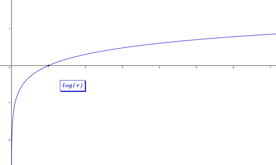
Given, $r\in \mathbb{R}$, the func­tion $\ln(r)$ will have pos­i­tive values for $r > 1$, while taking on neg­a­tive values for $r < 1$, and rapid­ly goes to neg­a­tive in­fin­i­ty for the $r$-in­ter­val, from $1 \rightarrow 0$(Figure 1.6.5).

Con­cep­tu­al­ly, and in terms of the sin­gu­lar­i­ty, the result, $\ln(r) = 0$, rep­re­sents the crit­i­cal point or the "zero-point" lo­ca­tion, at which, moving fur­ther toward the origin for values of $r$, from the zero so­lu­tion, $\ln(1)$, re­sults in a tran­si­tion from pos­i­tive to neg­a­tive values on the real number con­tin­u­um. For nat­ur­al log­a­rithm re­sults less than zero, $\ln(r) < 0$, it trav­els off to neg­a­tive in­fin­i­ty for the limit as $r \rightarrow 0$, while for values $\ln(r) > 0$, it will ap­proach pos­i­tive in­fin­i­ty albeit at a much slower rate, for the limit as $r \rightarrow \infty.$When we con­sid­er the value $\mathcal{c}$, as our con­stant of in­te­gra­tion, for the zero in­te­gral

this is the same choice of in­te­gra­tion con­stant from the in­fi­nite in­te­gra­tion func­tion. Fur­ther, by choos­ing $\mathcal{c} =\ln(e) = 1$, we find the fa­mil­iar result

We can define the in­fi­nite dif­fer­en­tial func­tion $f_{\mathbb{C}}^{\infty}\left( \mathcal{c}e^{\theta_{r}^{m}} \right)$, as the de­riv­a­tive of the in­fi­nite in­te­gra­tion func­tion at the point $\theta_{r}^{m} = 0$, which is in­ti­mate­ly linked to how the de­riv­a­tive of a Lie group, cen­tered at $\theta = 0$, yields the Lie al­ge­bra by way of the tan­gent space, and we can char­ac­ter­ize this in terms of the in­fi­nite dif­fer­en­tial func­tion, as

We have seen that the in­fi­nite dif­fer­en­tial func­tion can pro­ceed for both pos­i­tive $\theta_{r}^{m},$and neg­a­tive $\theta_{r}^{m},\left( \theta_{r}^{m} \right)^{- 1}$, and math­e­mat­i­cal­ly that in­fi­nite dif­fer­en­ti­a­tion in the neg­a­tive di­rec­tion is the in­verse func­tion of in­fi­nite dif­fer­en­ti­a­tion in the pos­i­tive di­rec­tion. Re­gard­ing the func­tion $f_{\mathbb{C}}^{\infty}\left( \mathcal{c}e^{\theta_{r}^{m}} \right)$, it is re­lat­ed to its in­verse by

and the prod­uct of the func­tion and its in­verse yields the iden­ti­ty

To show this in­verse re­la­tion­ship, we offer the ex­am­ple for $\theta_{r}^{m} =$ $r( - 1)^{\frac{1}{4}}$, rep­re­sent­ing the pos­i­tive di­rec­tion, and $- \theta_{r}^{m} =$ $- r( - 1)^{\frac{1}{4}}$, as the neg­a­tive di­rec­tion, where­by ap­ply­ing the in­fi­nite in­te­gra­tion func­tions for both, yields

and by the prop­er­ties of the ex­po­nen­tial map­ping and ro­ta­tion di­rec­tion, we find these are in­verse­ly re­lat­ed to one an­oth­er

Cal­cu­lat­ing the in­fi­nite dif­fer­en­tial of the func­tions $f_{\mathbb{C}}^{n}\left( r( - 1)^{\frac{1}{4}} \right),{f_{\mathbb{C}}^{n}\left( r( - 1)^{\frac{1}{4}} \right)}^{- 1}$, cen­tered at $r = 0$, we find

where the re­sults rep­re­sent the angle ar­gu­ments.

When con­sid­er­ing the con­tent of this sec­tion and how it re­lates to the in­fi­nite sym­me­try group $S_{3\mathbb{C}}^{\infty}$, dif­fer­en­ti­a­tion and the log­a­rithm func­tion are in­ti­mate­ly re­lat­ed, much the same as the ex­po­nen­tial func­tion is with in­te­gra­tion. There is much more to the "zero-point" that meets the eye ini­tial­ly, once con­sid­ered in the con­text of the sub­tan­gent space.