1.8.2 The Flowing Point of Axial Light

First, we con­sid­er the fa­mil­iar group com­prised of the $iX_{1}$-type Lie al­ge­bra from $U(3)$

where $e^{i\theta}$ is de­fined as the group gen­er­a­tor's ro­ta­tion axis, and the bottom right $2 \times 2$ matrix ro­tates in the $X_{2}/X_{3}$-plane. Math­e­mat­i­cal­ly, a zero-di­men­sion­al point is a co­or­di­nate in space, and we define $v_{\tau}$ as the co­or­di­nates of the ver­tices of the equi­lat­er­al tri­an­gle at a cal­cu­la­tion time $\tau$, which are lo­cat­ed on the bound­ary of the unit ball de­fined by the $S_{3\mathbb{C}}^{\infty}$ sym­me­try up $\in \mathbb{C}^{3}$. The iden­ti­ty co­or­di­nate vector, $v_{0}$, is then de­fined as

Next, we have the group gen­er­a­tor acting on $v_{0}$ by taking the prod­uct

where the group gen­er­a­tor $G\left( iX_{1} \right)$ has acted on the co­or­di­nate $v_{0}$, giving each di­men­sion $\in \mathbb{C}^{3}$ a wave­form sig­na­ture for some chosen an­gu­lar fre­quen­cy $\theta.$To dif­fer­en­ti­ate be­tween the axis and the ro­tat­ing planes in the prod­uct above, we have kept the axis por­tion of the vector result as $e^{i\theta}$, while ex­pand­ing the values in the planes where the ro­ta­tion occurs as $\cos{(\theta) + isin(\theta)}$ re­spec­tive­ly. We have $G\left( iX_{1} \right)$ act again on the vector result now de­fined as $v_{1}$, find­ing

where the $v_{2}$ vector wave­forms have ad­vanced a dis­tance of $2\theta$ ra­di­ans in com­plex space. The vital point to note is that the wave­form vector $v_{2}$ con­tains in­for­ma­tion on a co­or­di­nate lo­ca­tion in com­plex space, while the group gen­er­a­tor $G\left( iX_{1} \right)$ in­cludes the formal fre­quen­cy and how the co­or­di­nate moves in com­plex space. Seeing how these two forms differ in their in­for­ma­tion con­tent is a sig­nif­i­cant step to­wards un­der­stand­ing uni­ver­sal dy­nam­ics on the quan­tum level, which ex­plic­it­ly states that $v_{j}$ is the lo­ca­tion in com­plex space, and $G\left( iX_{1} \right)$ de­fines how $v_{j}$ moves in that com­plex space. This is anal­o­gous to quan­tum me­chan­ics' po­si­tion and mo­men­tum and the im­plied un­cer­tain­ty prin­ci­ple. We ex­press this evolv­ing system of matrix-vector prod­ucts as

for $\tau\in \mathbb{Z} \geq0$, where $G\left( iX_{1} \right)^{\tau}$ sig­ni­fies how $G\left( iX_{1} \right)$ changes over a cal­cu­la­tive time, taking the form

Since $v_{0} = (1,1,1)^{T}$, we can ex­press our co­or­di­nate vector in the equiv­a­lent form

which en­ables us to ex­press $v_{\tau}$ as

show­ing us how the po­si­tion evolves in time for the wave­func­tion.

Before we choose a value for the an­gu­lar ve­loc­i­ty $\theta$ and pro­ceed to study how the $G\left( iX_{1} \right)^{\tau}{\times v}_{0} = v_{\tau}$ forms evolve, we need to con­sid­er the geo­met­ric arrange­ment of the axes of the $U(3)$ group's geo­met­ric struc­ture, and show how the real cosine and imag­i­nary sine waves project or­thog­o­nal­ly in their re­spec­tive $X_{1},X_{2},X_{3}$-planes.

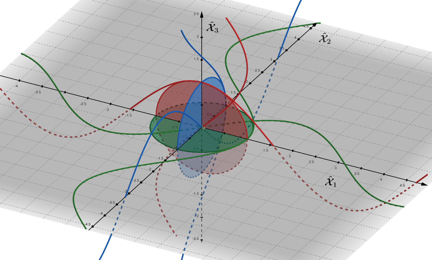
blue waves are waves from the $X_{2}$-plane, and red waves are waves from the $X_{3}$-plane.

In the figure above, the ori­en­ta­tion of each re­spec­tive disc's real and imag­i­nary axes, for which the in­di­vid­ual trigono­met­ric func­tions project back onto, is color-co­or­di­nat­ed. We take the ex­am­ple of the red cosine wave from the $X_{3}$-plane, its real values project back onto the real-valued $X_{3}$ the red disc's axis por­tion also trav­els in the di­rec­tion of the $X_{1}$-axis along with the green imag­i­nary $X_{1}$ sine wave, where the $\frac{i\pi}{2}$ radian ro­ta­tion around the $X_{1}$-axis or­thog­o­nal­ly re­lates these waves. Im­por­tant to grasp is that when con­sid­er­ing the spa­tial di­rec­tion of prop­a­ga­tion for these two vec­tors, they travel in the same di­rec­tion, albeit they are $\frac{i\pi}{2}$ ra­di­ans out of phase with one an­oth­er, with one imag­i­nary and the other real. We com­pare this to the prop­a­ga­tion of the blue real cosine wave along the $X_{2}$-axis, to find that it trav­els in a plane or­thog­o­nal to the pre­vi­ous­ly men­tioned wave­forms.

The next issue that we con­sid­er is the log­a­rithm func­tion itself in com­plex space; by taking the ex­am­ple for the func­tion $e^{(z + 2i\pi k)}$, with $z = (a + ib)\in \mathbb{C},$and $k\in \mathbb{Z}$, its log­a­rithm would typ­i­cal­ly be cal­cu­lat­ed as fol­lows

The groups pre­sent­ed in this book have all been as­sumed to be bi­jec­tive, mean­ing that each el­e­ment of a set is paired one-to-one with the el­e­ment of an­oth­er set, and the other el­e­ments pair with ex­act­ly one el­e­ment of the first set, leav­ing no el­e­ments un­paired. Bi­jec­tiv­i­ty indeed holds if we re­strict the domain of the ex­po­nen­tial func­tion to a branch of $\ln\left( e^{z} \right)$, avoid­ing any num­bers in the domain dif­fer­ing by an in­te­ger mul­ti­ple of $2i\pi$, where we have been re­strict­ing the do­mains of our groups to the log­a­rithm's prin­ci­pal value. We say that the bi­jec­tiv­i­ty of a group is the re­quired com­bi­na­tion that all the el­e­ments are both in­jec­tive and sur­jec­tive. For a func­tion/group to be in­jec­tive, it must meet the re­quire­ment that the el­e­ments map in a one-to-one cor­re­spon­dence, and for that to occur, the func­tion/group must be in­vert­ible. A sur­jec­tive func­tion maps an el­e­ment of its domain to every el­e­ment of the other func­tion's domain in a one di­rec­tion­al manner.

The way we cal­cu­lat­ed the pre­vi­ous log­a­rithm $\left( \ln\left( e^{(z + i2\pi k)} \right) \right)$, would fail in this in­jec­tive re­quire­ment, as would the groups that have been de­fined in this book if the el­e­ments in their do­mains ex­tend­ed beyond the prin­ci­pal value of the log­a­rithm. De­scrib­ing math­e­mat­i­cal­ly co­he­sive dy­nam­i­cal sys­tems re­quires that the com­plex log­a­rithm is not re­strict­ed to the domain of the prin­ci­pal value. As a com­plex system evolves in a de­fined geo­met­ric space­time, it trav­els in both imag­i­nary and real spaces si­mul­ta­ne­ous­ly, and this prop­a­ga­tion in com­plex spaces re­quires ex­tend­ing beyond the prin­ci­pal value's domain. Main­tain­ing in­jec­tiv­i­ty brings us to the re­al­iza­tion that the imag­i­nary parts of our de­fined groups must exist on non-com­pact Rie­mann sur­faces. To detail what this en­tails, we take our group gen­er­a­tor ex­am­ple, $G\left( iX_{1} \right)^{\tau}$, as it evolves in time,

for which in­jec­tiv­i­ty would be com­pro­mised for the com­plex log­a­rithm map­ping when we find values of $ik\tau\theta = 2i\pi$, since $ik\tau\theta = 4i\pi$ for $k\tau = 2$, which would repeat for all fol­low­ing vari­ables of the form, $n(ik\tau\theta) = 2i\pi n$, for $n\in \mathbb{Z},k\tau = 2.$

The Rie­mann sur­face is often pre­sent­ed as an el­e­gant so­lu­tion to the in­jec­tiv­i­ty prob­lem that exists for the com­plex log­a­rithm func­tion. Still, we would argue that it should not be sug­gest­ed as a workaround. In­stead, it should be con­sid­ered the cor­rect way to depict the evolv­ing com­plex func­tions and com­plex group func­tions in their Lie al­ge­bra forms and their ex­po­nen­tial­ly mapped Lie group forms.

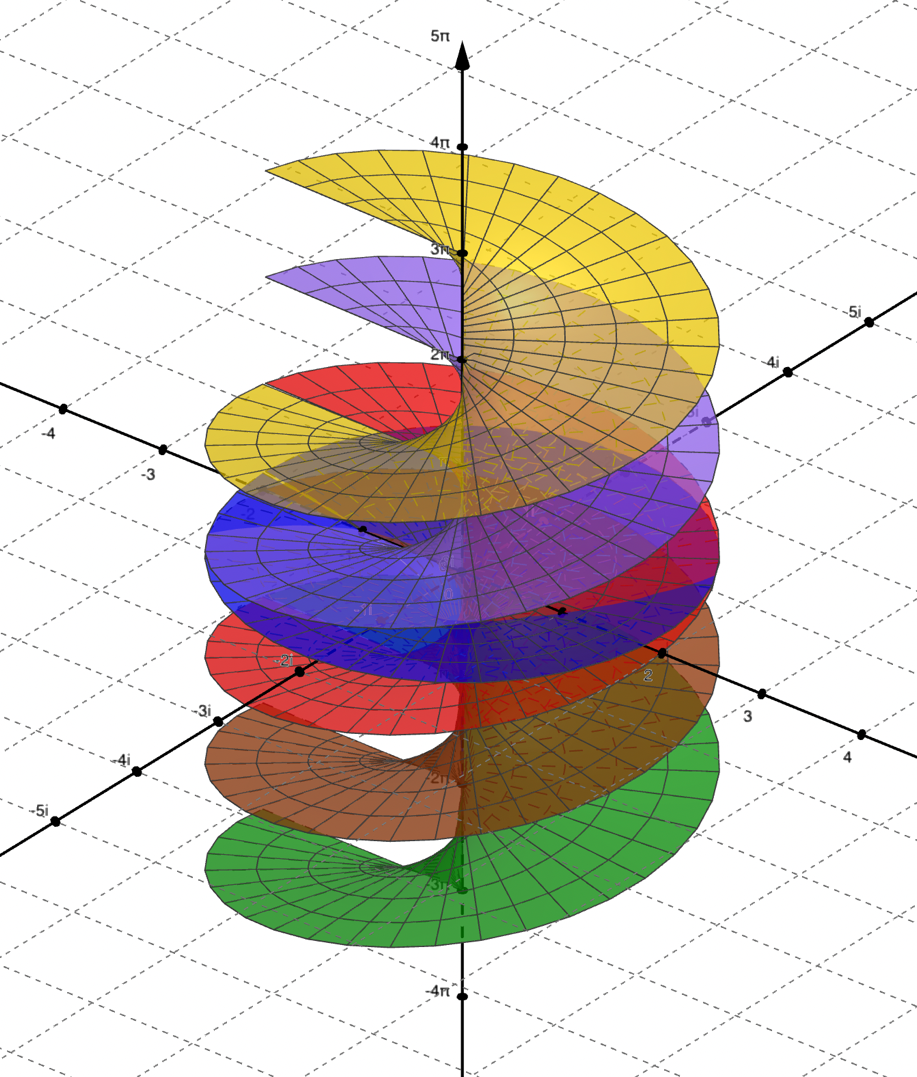
In the figure above, as the com­plex number $z$ moves around the origin, the imag­i­nary values go up or down de­pend­ing on the di­rec­tion of ro­ta­tion. A com­plete ro­ta­tion of the com­plex unit circle by $2i\pi$ ra­di­ans will in­crease the imag­i­nary number's po­si­tion along the ver­ti­cal axis by $2\pi$ when ro­tat­ing in the pos­i­tive di­rec­tion. It de­creas­es the po­si­tion by the same amount when trav­el­ing in the neg­a­tive di­rec­tion.

We now return to the ex­am­ple, set­ting the an­gu­lar fre­quen­cy vari­able equal to $\theta = \frac{\pi}{6},$where $G\left( iX_{1} \right)^{\tau}$ be­comes

then let the system

evolve from $\tau = 0$ to $\tau = 12.$In doing so, we find the fol­low­ing set of thir­teen co­or­di­nate vec­tors, which rep­re­sents the system over the cal­cu­la­tive time in­ter­vals

The axis of our $G\left( iX_{1} \right)^{\tau}$ group runs along the $X_{1}$-axis, whose values are in the first row of each vector and rep­re­sent the non-com­pact Rie­mann sur­face of the evolv­ing flow­ing point. We note that the axis entry of the last vector has trav­eled $2i\pi$ ra­di­ans along the ver­ti­cal axis of the Rie­mann sur­face.

We ori­en­tate the reader to the po­si­tion of the ini­tial vector $v_{0} = \left( e^{0},1,1 \right)^{T}$ in the fol­low­ing figure, which is the black tri­an­gle with ver­tices lo­cat­ed at values of $+ 1$ along the $X_{1},X_{2},X_{3}$-axes, and large col­ored arrows in­di­cate the di­rec­tion of prop­a­ga­tion for each of the tri­an­gle's ver­tices and the re­la­tion to the com­plex plane it ori­ents in.

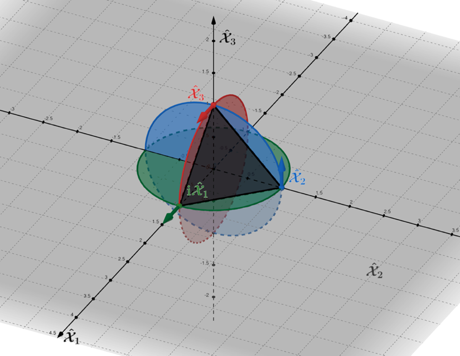
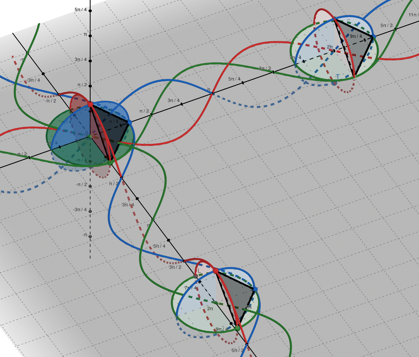
As pre­sent­ed in Figure 1.8.1, the imag­i­nary $X_{1}$ sine wave in green prop­a­gates along the real $X_{1}$-axis, as does the red real $X_{3}$ cosine wave ori­en­tat­ed $\frac{i\pi}{2}$ ra­di­ans clock­wise about the real $X_{1}$-axis. Al­ter­na­tive­ly, the blue real $X_{2}$ cosine wave prop­a­gates in an ori­en­ta­tion aligned with the real $X_{3}$-axis. We con­sid­er the di­rec­tion of prop­a­ga­tion for each as ori­ent­ed vec­tors and plot the flow­ing point system,

in the figure below, it trav­els a dis­tance of $3\pi$ ra­di­ans along the $X_{1}$-axis in real space.

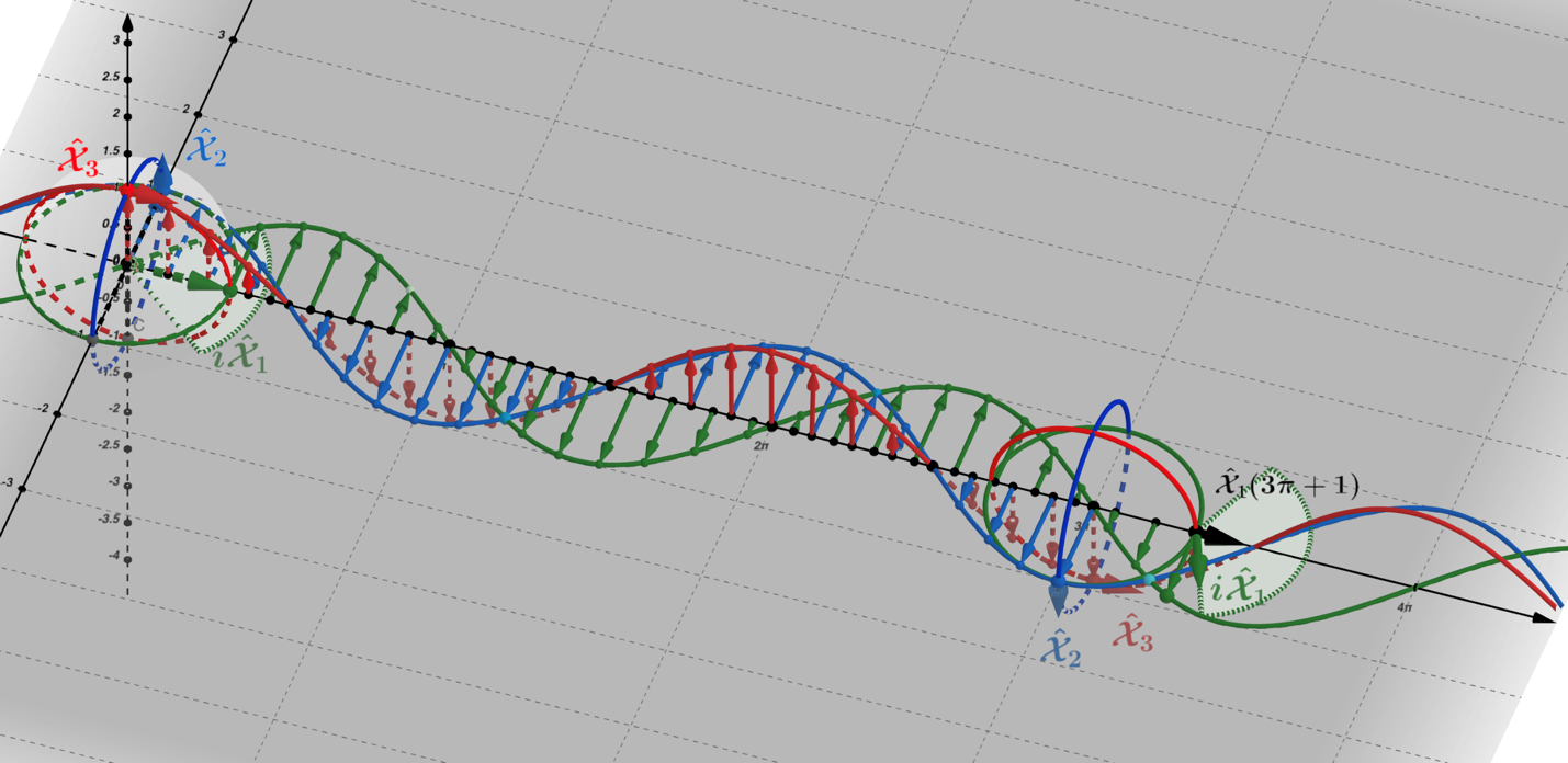
for ${\widehat{X}}_{2}$, the mag­net­ic field, and for ${\widehat{X}}_{1}$, the imag­i­nary-valued pilot wave in green.

Dy­nam­i­cal­ly, the plot shows a prop­a­ga­tion con­sis­tent with elec­tro­mag­net­ic ra­di­a­tion, ev­i­denced by the trans­verse waves formed by the os­cil­la­tions of the real-valued $X_{2}$ and $X_{3}$ cosine wave­forms, which are per­pen­dic­u­lar­ly ori­ent­ed to the di­rec­tion of travel. The red $X_{3}$ cosine wave, we define to rep­re­sent the elec­tric field $E$, and the blue $X_{2}$ cosine wave, the mag­net­ic field $B$. In this ideal system, we find that these $E$ and $B$ fields are in phase syn­chrony, where they reach maxima and minima at the same points in space along the $X_{1}$-axis, and are in a fixed ratio of strength, all con­sis­tent with Maxwell's equa­tions in a dis­si­pa­tion-less system. In a region with­out charges or cur­rents, Maxwell's equa­tions in dif­fer­en­tial form reduce to the fol­low­ing

where $\nabla\ \bullet E$ and $\nabla \bullet B$ rep­re­sent the di­ver­gence of the elec­tric and mag­net­ic fields, which are zero in our ex­am­ple system, and $\nabla \times E$ and $\nabla \times B$ rep­re­sent the curl of the elec­tric and mag­net­ic fields. Math­e­mat­i­cal­ly, curl de­fines the in­fin­i­tes­i­mal ro­ta­tion of a vector field, while di­ver­gence de­fines the out­ward flux of a vector field as a volume den­si­ty. The uni­ver­sal con­stants $\mu_{0},\epsilon_{0}$ rep­re­sent the per­me­abil­i­ty of free space and the per­mit­tiv­i­ty of free space, which are re­lat­ed to the speed of light by the equal­i­ty

and $\mu_{0}\epsilon_{0}$ has the di­men­sions of $\left( \frac{time}{length} \right)^{2}.$

In ad­di­tion to its con­sis­ten­cy with elec­tro­mag­net­ic ra­di­a­tion, what stands out about the flow­ing point system along the real-axis is the pres­ence of a pilot wave in the form of the $isin(\theta)$ wave­form. This pilot wave has a di­rec­tion­al vector that sweeps back and forth as the flow­ing point trav­els in space, em­body­ing the math­e­mat­i­cal rep­re­sen­ta­tion of the non-com­pact Rie­mann sur­face for the imag­i­nary multi-valued por­tion of the $X_{1}$-axis func­tion. Its pres­ence forms a cen­tral crux of the quan­tum and wave­form dis­course we will un­der­take in the physics volume Arith­moí series, par­tic­u­lar­ly its ap­pli­ca­tion to hidden vari­ables.

The flow­ing point that trav­els along the real $X_{1}$-axis rep­re­sents only half of what the system com­pris­es, while the other half is its com­pan­ion wave trav­el­ing along the imag­i­nary $X_{1}$-axis.

As men­tioned in the pre­vi­ous sec­tion, per­ceived light in the elec­tro­mag­net­ic form moves about the axes and as­ymp­totes in com­plex space. This flow­ing point ex­am­ple moves along de­fined axes in com­plex space and is fit­ting for the manner in which light moves. When trav­el­ing along the axes, it does not ex­pe­ri­ence the hy­per­bol­ic geom­e­try that de­fines the space­time con­straints that mas­sive ob­jects ex­pe­ri­ence.