1.6.5 Outer Products and Infinities

Math­e­mati­cians and physi­cists tend to reduce math­e­mat­ics equa­tions into the sim­plest and most com­pact forms, but some­times taking an ex­pand­ed ap­proach to these equa­tions can yield valu­able in­sights, hint­ing at an el­e­gant struc­ture in the math­e­mat­ics that might have oth­er­wise been ob­scured by re­duc­tion­ism.

An outer prod­uct is the prod­uct of two co­or­di­nate vec­tors that form a matrix and is re­lat­ed to tensor al­ge­bra. If we have two vec­tors $\widehat{u_{i}},\ \widehat{v_{j}}$, for ${\widehat{u}}_{i}$, a column vector and ${\widehat{v}}_{j}$, a row vector, their tensor prod­uct, as $\widehat{u}\bigotimes_{}^{}\widehat{v}$, is an $i \times j$ matrix, $w_{ij}$. So, for vec­tors ${\widehat{u}}_{i} = \left( a_{1},\ a_{2},\ a_{3},\ a_{4} \right)^{T}$, ${\widehat{v}}_{j} = \left( b_{1},\ b_{2},\ b_{3},\ b_{4} \right)$, their tensor prod­uct is

An im­por­tant dis­tinc­tion, re­vers­ing the order of vec­tors in the outer prod­uct will result in a dif­fer­ent matrix result. The matrix re­sults will have de­ter­mi­nants equal to zero, for outer prod­ucts formed by two vec­tors of the same di­men­sions greater than one. Ten­sors are vital to math­e­mat­i­cal physics and are used fre­quent­ly in quan­tum me­chan­ics to de­scribe quan­tum system in­ter­ac­tions very well, where the goal in their use is to de­scribe how basic things in­ter­act with one an­oth­er.

When it comes to the in­fi­nite series that en­com­pass­es the ex­po­nen­tial map­ping in Lie theory, tensor al­ge­bras can be con­sid­ered by taking these in­fi­nite series to be co­or­di­nate vec­tors. By doing so, we can take a more ex­pan­sive look at how these in­fi­nite math­e­mat­i­cal forms in­ter­act with each other. The in­fi­nite series that con­verges to $e^{ix}$, is com­posed of two dis­tinct in­fi­nite series, the in­fi­nite power series and rec­i­p­ro­cal fac­to­r­i­al series, whose dot prod­uct leads to Euler's for­mu­la

Euler's for­mu­la is com­posed of a geo­met­ric series por­tion, being

and the rec­i­p­ro­cal fac­to­r­i­al series por­tion

From the two dis­tinct series, we set $u_{m}$ equal to the sum of the geo­met­ric power series

and $v_{n}$, as the sum of the in­fi­nite rec­i­p­ro­cal fac­to­r­i­al series

We define the column vector ${\widehat{u}}_{m}$, and the row vector ${\widehat{v}}_{n}$, as in­fi­nite-di­men­sion­al, com­posed of the el­e­ments from $u_{m},v_{n}$

and the outer prod­uct of these vec­tors $\widehat{u} \otimes \widehat{v}$, form the matrix $X$

The first thing that stands out is that the trace of the $X$ matrix, $tr(X)$, shown as the bold el­e­ments along the main di­ag­o­nal, is the in­fi­nite series for $e^{ix}$, $tr(X) = e^{ix}$. In terms of the eigen­val­ues and eigen­vec­tors of the $X$matrix, there is a single eigen­val­ue $\lambda$, equal to $e^{ix}$

that would be in an eigen­val­ue matrix $D$, in the row/column po­si­tion $d_{\infty,\infty}$. Note­wor­thy, is that the eigen­val­ue $\lambda = e^{ix}$, can take on an in­fi­nite number of values for any ar­gu­ment for $x\in \mathbb{R}$, on the unit circle, en­com­pass­ing the essence of Lie theory and the in­fin­i­tes­i­mal ro­ta­tions. In con­trast to the lone eigen­val­ue, there are an in­fi­nite number of eigen­vec­tors ${\widehat{v}}_{i}$, rep­re­sent­ing the columns in the eigen­vec­tor matrix $V$

The eigen­vec­tor columns in $V$, except for the last column, arrange in a pat­tern con­sis­tent with the first row equal­ing the fac­to­r­i­al el­e­ment $- \frac{1}{k!}$, for $k$, the column number, and the number one in the row number $j = k + 1$. The last eigen­vec­tor column as a sum, rep­re­sents a geo­met­ric power series, which, for $|x| > 1$, con­verges to

If we return and con­sid­er the in­fi­nite sum of the el­e­ments $\in X$, it is easily seen that each row in the matrix will sum to $e(ix)^{j - 1}$, for $j,$the row number. This leads to a con­ver­gent in­fi­nite row sum for $X$, when $|x| < 1$

and is con­sis­tent with the prod­uct result we would find be­tween the sum­ma­tion of the vector el­e­ments from $\widehat{u_{i}},\ \widehat{v_{j}}$

From the stand­point of matrix theory, the el­e­ments on the main di­ag­o­nal rep­re­sent the sym­met­ric por­tion of the prod­uct $\widehat{u} \otimes \widehat{v}$, which sum to $e^{ix}$, while other el­e­ments then rep­re­sent the an­ti­sym­met­ric por­tion of the prod­uct. Taken to­geth­er, the sym­met­ric and an­ti­sym­met­ric el­e­ments are prod­uct rep­re­sen­ta­tions for every el­e­ment in each in­fi­nite series with one an­oth­er, rep­re­sent­ing columns, rows, and off-di­ag­o­nals, which are also in­fi­nite series. To better un­der­stand the sym­met­ric, and asym­met­ric por­tions of $X$, it is im­por­tant to re­al­ize that $\widehat{u} \otimes \widehat{v} \neq \widehat{v} \otimes \widehat{u}$, mean­ing our vec­tors are non-com­mu­ta­tive as outer prod­ucts. This be­comes clear by show­ing an ab­bre­vi­at­ed ver­sion of the outer prod­uct matrix $\widehat{v} \otimes \widehat{u}$,

for which the el­e­ments on the main di­ag­o­nal are the same as the first outer prod­uct $\widehat{u} \otimes \widehat{v}$, defin­ing the sym­met­ric por­tion.

The an­ti­sym­met­ric por­tion of $\widehat{v} \otimes \widehat{u},$are the non-di­ag­o­nal el­e­ments $\in X^{'}$, and are trans­posed in com­par­i­son to those in $X$. This leads us back to the geo­met­ric prod­uct of vec­tors, to con­sid­er its sym­met­ric dot prod­uct and an­ti­sym­met­ric wedge prod­uct in terms of our in­fi­nite vector func­tion's outer prod­uct. The trace of our outer prod­uct matrix is con­sis­tent with an inner prod­uct, and could also be for the dot prod­uct, if we were to define the vec­tors as in­fi­nite in their co­or­di­nates. To con­sid­er the wedge prod­uct in re­la­tion to the outer prod­uct $X$, we con­sid­er the ex­pres­sion that re­lates the wedge to outer prod­uct

which, for the dif­fer­ence of outer prod­ucts should remind us of the com­mu­ta­tor op­er­a­tion. So, in terms of a geo­met­ric al­ge­bra analog, we can ex­press the geom­e­try prod­uct of the vec­tors $\widehat{u},\widehat{v},$as

which re­sults in

in which, the sym­met­ric por­tion of the outer prod­uct ma­tri­ces $X,X'$, van­ish­es in their dif­fer­ence, and we now have ad­di­tive in­verse re­la­tion­ships be­tween en­tries and their trans­pos­es. Given this ad­di­tive in­verse re­la­tion­ship, we now find the grand sum of the en­tries $\in$ $\mathrm{X}$, equals zero.

Re­turn­ing to the $X$ matrix, we can apply matrix group theory to our ex­po­nen­tial series tensor, by defin­ing a di­ag­o­nal­ized matrix $D$, rep­re­sent­ing the di­ag­o­nal el­e­ments $\in$ X

We en­ter­tain the matrix-prod­uct $D^{- 1}X$ , to find the re­sult­ing matrix $S$, which is a com­po­si­tion of in­vers­es $\in \mathbb{C}$, given that each entry's trans­pose is its in­verse, and this is a bi­jec­tive map­ping, with a matrix prod­uct in­verse $SD = X.$

A closer look at the $S$-matrix re­veals the con­ver­gence de­tails of the power series por­tion $\sum_{n = 0}^{\infty}(ix)^{n}$, from the func­tion $e^{ix}$, having a radius of con­ver­gence $|x| < 1$, for which we define $s$, as

and the limit, as $x \rightarrow 1$, as

In the limit $\lim_{x \rightarrow 1}{s(x)}$, we find a result which rep­re­sents the per­fect bal­ance of real and imag­i­nary num­bers, fit­ting the de­f­i­n­i­tion of a cone number from Chap­ter 4. The radius of con­ver­gence for values of $|x| < 1$, holds for the columns formed by en­tries in the lower-left tri­an­gle of the $S$-matrix. The main di­ag­o­nal, com­posed of ones, rep­re­sents the crit­i­cal point of the com­plex unit circle's bound­ary, which leads to the con­ver­gence radius tran­si­tion for the func­tion $e^{ix}$, rep­re­sent­ed by the el­e­ments in the upper-right tri­an­gle, hold­ing for $|x| > 1$.

The notion of an un­ex­tend­ed state and the tran­si­tion to an ex­tend­ed one, are math­e­mat­i­cal­ly present in this outer prod­uct matrix ex­am­ple, rem­i­nis­cent of con­cepts re­lat­ed to the in­fi­nite sphere of tan­gents spaces. This notion par­al­lels the log­a­rithm func­tion $\ln(x)$, from Figure 1.6.5, and the real number sign tran­si­tion oc­cur­ring at $\ln(1) = 0$, the point where the func­tion's curve breach­es the hor­i­zon­tal axis.

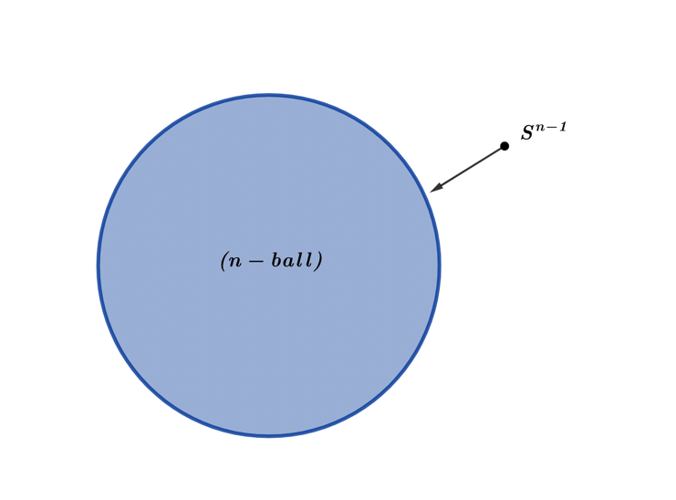
Math­e­mat­i­cal­ly speak­ing, a sphere is the bound­ary rep­re­sen­ta­tion of a ball, where the n-ball is de­fined by its $n$ number of di­men­sions and bound­ed by an (n-1) sphere. The $2$-ball, de­pict­ed below in Figure 1.6.9, has for its bound­ary the $1$-sphere $\in \mathbb{C}$, rep­re­sent­ing the $U(1)$ group.

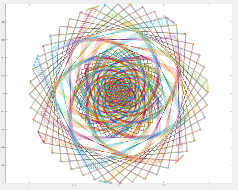
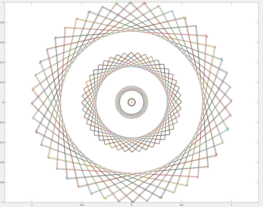
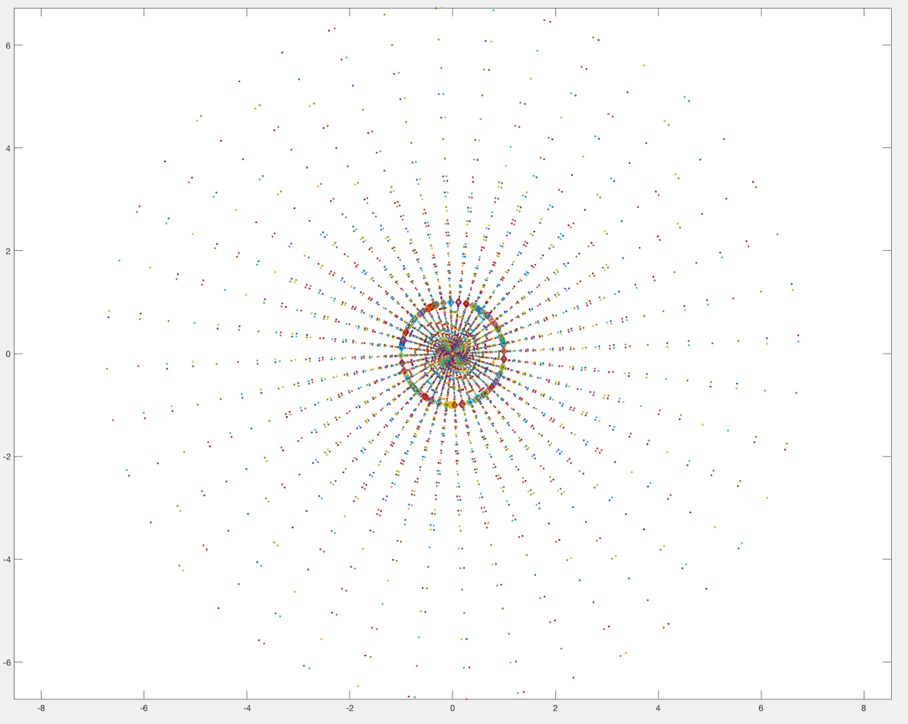
We can vi­su­al­ize the un­ex­tend­ed state, the ex­tend­ed state, and their phase tran­si­tion by plot­ting the values $x_{j} = \{ 0.9,\ 1.0,\ 1.1\}$, to rep­re­sent the nu­mer­i­cal phase tran­si­tion in the neigh­bor­hood of the crit­i­cal point at $\ln(x) = 0$. By taking suc­ces­sive powers of the outer prod­uct matrix $X = \ \widehat{u} \otimes \widehat{v}$, for $n = 60$ it­er­a­tions, we are cal­cu­lat­ing the outer prod­uct equiv­a­lent to taking suc­ces­sive powers of $\left( e^{ix} \right)^{n}\ = e^{ixn}$. This has the effect of ad­vanc­ing the point on the com­plex unit circle by $x_{j}$ ra­di­ans for each power it­er­a­tion, for which, the di­ag­o­nal en­tries will remain on the 2-ball's bound­ary.

The un­ex­tend­ed phase plot for $x_{j} = 0.9$, is seen in Figure 1.6.10, where the di­a­mond points on the unit circle rep­re­sent the el­e­ments of the $trace(X) = e^{ix}$. Lines con­nect each point to dis­cern the path that el­e­ment takes during each ro­ta­tion. The points are either on the bound­ary of the disc or inside the disc, given that $\left| x_{j} \right| < 1$, and is topo­log­i­cal­ly de­fined as closed.

The phase tran­si­tion occurs at the crit­i­cal point, when $x_{j} = 1.0$ (Figure 1.6.11), which rep­re­sents the bound­ary be­tween non-ex­ten­sion and ex­ten­sion, where the tran­si­tion is ev­i­denced by the mor­pho­log­ic change of pat­tern in the closed topol­o­gy, to that of re­peat­ing ring shapes em­a­nat­ing from the center of the 2-ball, ex­tend­ing to its bound­ary.

This math­e­mat­i­cal phase tran­si­tion can be con­sid­ered as the min­i­mal an­gu­lar fre­quen­cy nec­es­sary to extend beyond the bound­ary of the 2-ball. The ex­tend­ed-phase for $x = 1.1$, is plot­ted in Figure 1.6.12, where ray-like spin­dles extend past the ring of di­a­monds rep­re­sent­ing the 2-ball's bound­ary.

We can take the outer prod­uct a step fur­ther, by ap­ply­ing it to the matrix groups we have been study­ing, and in par­tic­u­lar, the outer prod­ucts of the in­fi­nite series rep­re­sen­ta­tions for non-com­mu­ta­tive al­ge­bras. We take $e^{X}$, to be the matrix ex­po­nen­tial of the $X_{1}$-type Lie al­ge­bra, and $e^{Y}$, the matrix ex­po­nen­tial of the $X_{2}$-type, for $e^{X} = \theta_{1}^{\left( 3,X_{1} \right)} = e^{\left( i\theta_{\left( 3,X_{1} \right)} \right)},$and $e^{Y} = \theta_{1}^{\left( 3,X_{2} \right)} = e^{\left( i\theta_{\left( 3,X_{2} \right)} \right)}$. We can then present the groups $e^{X},e^{Y}$, as the fol­low­ing in­fi­nite matrix ex­po­nen­tial series

We know that the prod­ucts $X^{n}Y^{k} \neq Y^{k}X^{n}$, for $n \times k = odd$, will not com­mute, where­as, $X^{n}Y^{k} = Y^{k}X^{n}$ will com­mute for $n \times k = even$, since even powers of the ma­tri­ces $X,Y$ will only have en­tries on the main di­ag­o­nal, en­sur­ing prod­uct com­mu­ta­tiv­i­ty. We form the $Z$-matrix by the outer prod­uct of the vec­tors $\widehat{X},\widehat{Y}$, which rep­re­sent the in­fi­nite series for $e^{X},e^{Y}$, as

and the matrix group prod­uct $e^{X}e^{Y} = e^{Z}$, as the grand sum of the outer prod­uct el­e­ments $\sum_{}^{}{\widehat{X} \otimes \widehat{Y}}$.

Main­tain­ing the matrix prod­uct arrange­ment is im­por­tant for $XY,$as $X$ and $Y$ do not nec­es­sar­i­ly com­mute, as seen for the $Z$-matrix in Figure 1.6.13. Our at­ten­tion should be drawn to the trace of $Z$, $tr(Z)$, which rep­re­sents the fol­low­ing in­fi­nite series

and if $X,Y$, com­mute, $XY = YX$, the series is a so­lu­tion of the mod­i­fied Bessel func­tion of the first kind

$$\left( \begin{array}{r} \begin{matrix} \mathbf{X}^{\mathbf{0}}\mathbf{Y}^{\mathbf{0}} & X^{0}Y^{1} & \frac{X^{0}Y^{2}}{2!} & \frac{X^{0}Y^{3}}{3!} & \frac{X^{0}Y^{4}}{4!} & \frac{X^{0}Y^{5}}{5!} & \frac{X^{0}Y^{6}}{6!} & \ldots & \frac{X^{0}Y^{\infty - 1}}{(\infty - 1)!} & \frac{X^{0}Y^{\infty}}{\infty!} \\ X^{1}Y^{0} & \mathbf{X}^{\mathbf{1}}\mathbf{Y}^{\mathbf{1}} & \frac{X^{1}Y^{2}}{2!} & \frac{X^{1}Y^{3}}{3!} & \frac{X^{1}Y^{4}}{4!} & \frac{X^{1}Y^{5}}{5!} & \frac{X^{1}Y^{6}}{6!} & \ldots & \frac{X^{1}Y^{\infty - 1}}{(\infty - 1)!} & \frac{X^{1}Y^{\infty}}{\infty!} \\ \frac{X^{2}Y^{0}}{2!} & \frac{{X^{2}Y}^{1}}{2!} & \frac{{\mathbf{X}^{\mathbf{2}}\mathbf{Y}}^{\mathbf{2}}}{(\mathbf{2}!)(\mathbf{2}!)} & \frac{{X^{2}Y}^{3}}{(3!)(2!)} & \frac{{X^{2}Y}^{4}}{(4!)(2!)} & \frac{{X^{2}Y}^{5}}{(5!)(2!)} & \frac{{X^{2}Y}^{6}}{(6!)(2!)} & \ldots & \frac{X^{2}Y^{\infty - 1}}{(\infty - 1)!2!} & \frac{X^{2}Y^{\infty}}{(\infty!)(2!)} \\ \frac{X^{3}Y^{0}}{3!} & \frac{{X^{3}Y}^{1}}{3!} & \frac{{X^{3}Y}^{2}}{(2!)(3!)} & \frac{{\mathbf{X}^{\mathbf{3}}\mathbf{Y}}^{\mathbf{3}}}{(\mathbf{3}!)(\mathbf{3}!)} & \frac{{X^{3}Y}^{4}}{(4!)(3!)} & \frac{{X^{3}Y}^{5}}{(5!)(3!)} & \frac{{X^{3}Y}^{6}}{(6!)(3!)} & \ldots & \frac{X^{3}Y^{\infty - 1}}{(\infty - 1)!3!} & \frac{X^{3}Y^{\infty}}{(\infty!)(3!)} \\ \frac{X^{4}Y^{0}}{4!} & \frac{{X^{4}Y}^{1}}{4!} & \frac{{X^{4}Y}^{2}}{(2!)(4!)} & \frac{X^{4}Y^{3}}{(3!)(4!)} & \frac{{\mathbf{X}^{\mathbf{4}}\mathbf{Y}}^{\mathbf{4}}}{(\mathbf{4}!)(\mathbf{4}!)} & \frac{{X^{4}Y}^{5}}{(5!)(4!)} & \frac{{X^{4}Y}^{6}}{(6!)(4!)} & \ldots & \frac{X^{4}Y^{\infty - 1}}{(\infty - 1)!4!} & \frac{X^{4}Y^{\infty}}{(\infty!)(4!)} \\ \frac{X^{5}Y^{0}}{5!} & \frac{{X^{5}Y}^{1}}{5!} & \frac{{X^{5}Y}^{2}}{(2!)(5!)} & \frac{{X^{5}Y}^{3}}{(3!)(5!)} & \frac{{X^{5}Y}^{4}}{(4!)(5!)} & \frac{{\mathbf{X}^{\mathbf{5}}\mathbf{Y}}^{\mathbf{5}}}{(\mathbf{5}!)(\mathbf{5}!)} & \frac{{X^{5}Y}^{6}}{(6!)(5!)} & \ldots & \frac{X^{5}Y^{\infty - 1}}{(\infty - 1)!5!} & \frac{X^{5}Y^{\infty}}{(\infty!)(5!)} \\ \frac{X^{6}Y^{0}}{6!} & \frac{{X^{6}Y}^{1}}{6!} & \frac{{X^{6}Y}^{2}}{(2!)(6!)} & \frac{{X^{6}Y}^{3}}{(3!)(6!)} & \frac{{X^{6}Y}^{4}}{(4!)(6!)} & \frac{{X^{6}Y}^{5}}{(5!)(6!)} & \frac{{\mathbf{X}^{\mathbf{6}}\mathbf{Y}}^{\mathbf{6}}}{(\mathbf{6}!)(\mathbf{6}!)} & \ldots & \frac{X^{6}Y^{\infty - 1}}{(\infty - 1)!6!} & \frac{X^{6}Y^{\infty}}{(\infty!)(6!)} \\ \mathbf{\vdots} & \vdots & \vdots & \vdots & \vdots & \vdots & \vdots & \mathbf{\ddots} & \vdots & \vdots \\ \frac{X^{\infty - 1}Y^{0}}{(\infty - 1)!} & \frac{X^{\infty - 1}Y^{1}}{(\infty - 1)!} & \frac{X^{\infty - 1}Y^{2}}{2!(\infty - 1)!} & \frac{X^{\infty - 1}Y^{3}}{3!(\infty - 1)!} & \frac{X^{\infty - 1}Y^{4}}{4!(\infty - 1)!} & \frac{X^{\infty - 1}Y^{5}}{5!(\infty - 1)!} & \frac{X^{\infty - 1}Y^{6}}{6!(\infty - 1)!} & \ldots & \frac{\mathbf{X}^{\mathbf{\infty - 1}}\mathbf{Y}^{\mathbf{\infty - 1}}}{\left( \mathbf{\infty - 1} \right)\mathbf{!}\left( \mathbf{\infty - 1} \right)\mathbf{!}} & \frac{X^{\infty - 1}Y^{\infty}}{\infty!(\infty - 1)!} \\ \frac{X^{\infty}Y^{0}}{\infty!} & \frac{X^{\infty}Y^{1}}{\infty!} & \frac{X^{\infty}Y^{2}}{(2!)(\infty!)} & \frac{X^{\infty}Y^{3}}{(3!)(\infty!)} & \frac{X^{\infty}Y^{4}}{(4!)(\infty!)} & \frac{X^{\infty}Y^{5}}{(5!)(\infty!)} & \frac{X^{\infty}Y^{6}}{(6!)(\infty!)} & \ldots & \frac{X^{\infty}Y^{\infty - 1}}{(\infty - 1)!\infty!} & \frac{\mathbf{X}^{\mathbf{\infty}}\mathbf{Y}^{\mathbf{\infty}}}{\left( \mathbf{\infty!} \right)\left( \mathbf{\infty!} \right)} \end{matrix} \end{array} \right)$$

The mod­i­fied Bessel func­tion of the first kind $I_{n}(x)$, for $n = 0$, is the so­lu­tion of the fol­low­ing mod­i­fied Bessel dif­fer­en­tial equa­tion

and these func­tions rep­re­sent the radial com­po­nents of the vi­bra­tion modes on the cir­cu­lar drum. To vi­su­al­ize the Bessel func­tion, we take the outer prod­uct $\widehat{X} \otimes \widehat{Y}$, for two $U(1)$Lie groups with vari­ables $X = ix,Y = iy,$to yield a Bessel func­tion of the first kind, as

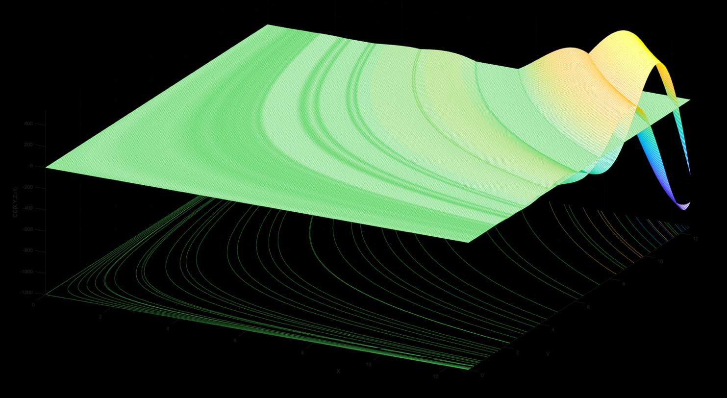
In Figure 1.6.14 we plot this Bessel func­tion for both its real and imag­i­nary radial com­po­nents, where wave forms can be seen prop­a­gat­ing along the sur­face of the drum and dis­pers­ing as the dis­tance from the im­pulse in­creas­es.

The $Z$-matrix can also be mul­ti­plied on the left by the in­verse di­ag­o­nal com­po­nents of $X,$ ${(D}_{X} \times Z)$, and mul­ti­plied on the right by the in­verse di­ag­o­nal com­po­nents of $Y,{(Z \times D}_{Y})$, for $D_{X},D_{Y}$ de­fined, as

to find the fol­low­ing two-vari­able tan­gent space field matrix $S_{XY}$, com­posed of $X,Y$

and the matrix $S_{XY}$, is like the outer-prod­uct matrix $S$ in Eq. 1.6.135, having en­tries with in­vers­es for their trans­pos­es. We define the fol­low­ing non-com­mut­ing ma­tri­ces $X,Y$

for $X = \theta_{r}^{\left( 3,X_{1} \right)} = r_{X_{1}}e^{i\theta_{\left( 3,X_{1} \right)}}$, and $Y = \theta_{r}^{\left( 3,X_{2} \right)} = {r_{X_{2}}e}^{i\theta_{\left( 3,X_{2} \right)}}$, The fol­low­ing prod­ucts would result:

for $I_{3}$, the $3 \times 3$ iden­ti­ty matrix, and $Y_{2},Y_{3}$, the $Y$-type cyclic matrix groups. A prod­uct ex­am­ple in­volv­ing $X,Y$, is the Lie al­ge­bra prod­uct ${X^{- 3}Y}^{3}X^{3}Y^{- 3}$, which will gen­er­ate the fol­low­ing $Y_{2}$-type matrix

given $n$, odd-valued, and the $X^{- n}Y^{n}X^{n}Y^{- n}$ prod­uct arrange­ment. The evenly dis­trib­uted $r$ terms could have also been omit­ted in the matrix result, since they are evenly dis­trib­uted in the nu­mer­a­tor and de­nom­i­na­tors and cancel in each ra­tio­nal. Each entry in the field $S_{XY}$, is com­prised of tan­gent space el­e­ments for their ar­gu­ments, which can be ap­pre­ci­at­ed by eval­u­at­ing the prod­uct for the $S_{XY(2,1)}$ entry, $X^{- 1}Y^{1}$,

where the in­verse al­ge­bra el­e­ments $X^{- 1}$ rotate in the op­po­site di­rec­tion to the $Y^{1}$ al­ge­bra. So, the matrix $X^{- 1}Y^{1}$, can be thought of as a su­per­po­si­tion of the Lie al­ge­bras $\in X^{- 1},Y^{1}$, in the ex­po­nen­tial, mul­ti­plied by ratios of the al­ge­bra vari­ables $\left( \frac{r_{X_{2}(j)}}{r_{X_{1}(j)}} \right)$, as lead­ing co­ef­fi­cients. Math­e­mat­i­cal­ly we can con­cep­tu­al­ize the outer prod­uct $e^{X} \otimes e^{Y}$, as a field formed, as $S_{XY}$, in which the Lie groups $e^{X},\ e^{Y}$ op­er­ate in.

Con­cep­tu­al­ly, we can see move­ment in the $S_{XY}$ field, by taking it­er­a­tion prod­ucts for $X$, on the left, and $Y$, on the right, to map or trans­form from a start­ing po­si­tion to an end po­si­tion. For ex­am­ple, the fol­low­ing se­quence of prod­ucts takes us from a start­ing point at $\mathbf{X}^{- \mathbf{1}}\mathbf{Y}^{\mathbf{1}}$, to the end po­si­tion at $\mathbf{X}^{\mathbf{2}}\mathbf{Y}^{- \mathbf{2}}$:

This move­ment se­quence is shown in bold with di­rec­tion­al arrows, rep­re­sent­ing the path-con­nec­tion

As a whole, move­ment in the outer prod­uct field $Z = \widehat{X} \otimes \widehat{Y}$, occurs by di­rec­tion­al in­te­gra­tion and dif­fer­en­ti­a­tion, where sim­i­lar to our pre­vi­ous ex­am­ple; from a start­ing point at $X^{- 1}Y^{1} \in Z$, moving three field po­si­tions to the right is the result of three in­te­gra­tions of $X^{0}Y^{1}$with re­spect to $X$, which, as­sum­ing no con­stants of in­te­gra­tion, is

Next, by taking the par­tial de­riv­a­tive, $\partial Y$, of this in­te­gral result, the field po­si­tion shifts upward by one

and the path-con­nect­ed move­ment se­quence is shown in bold in the $Z$-matrix, as

Math­e­mat­i­cal­ly speak­ing, move­ment in the $Z$-matrix away from the iden­ti­ty at $\epsilon = X^{0}Y^{0}$ is an­a­lyt­i­cal­ly con­ver­gent, since its basis is rooted in the ab­solute con­ver­gence of the ex­po­nen­tial series. So, the limits as $n \rightarrow \infty$, for in­fi­nite in­te­gra­tions to the right $(dX)$, down­ward $(dY)$, and di­ag­o­nal­ly $(dXdY)$, all con­verge to zero

This holds, given the sum of el­e­ments for any row, column, or di­ag­o­nal, con­verge to an ex­po­nen­tial map­ping of Lie al­ge­bras $X,Y$, in varied pro­por­tions. Dif­fer­en­tial move­ment toward the origin is anal­o­gous to its in­te­gra­tion coun­ter­part, where the re­spec­tive limits will all con­verge to the iden­ti­ty $\epsilon$, for $n,m,(n,m) \rightarrow 0.$

We have seen that the Baker-Camp­bell-Haus­dorff for­mu­la ex­press­es the matrix log­a­rithm for the prod­uct of two matrix groups as an in­fi­nite series of nested Lie brack­ets

and the outer prod­uct of two matrix groups in in­fi­nite series form $e^{X} \otimes e^{Y}$, rep­re­sents the result $e^{X}e^{Y} = e^{Z}$, as the sum­ma­tion of an in­fi­nite number of com­mu­ta­tive and or non-com­mu­ta­tive Lie al­ge­bras

The sum­ma­tion above can be de­fined by a bi­no­mi­al fac­to­r­i­al series, from the well-known bi­no­mi­al the­o­rem

with the ex­cep­tion that the rec­i­p­ro­cal fac­to­r­i­al series is present in the de­nom­i­na­tor, and we must keep in mind that $X,Y$, will not nec­es­sar­i­ly com­mute as they are typ­i­cal­ly treat­ed in the com­bi­na­torics of com­mut­ing bi­no­mi­al theory. Ap­ply­ing the outer prod­uct ap­proach to the matrix log­a­rithm also en­ables us to study the fields that they form. By choos­ing vec­tors de­fined by the log­a­rithm func­tion's in­fi­nite series

we set the vector $\widehat{u}$ to be the geo­met­ric series in the nu­mer­a­tor, and the vector $\widehat{v}$ to be the al­ter­nat­ing har­mon­ic series

We take the outer prod­uct of these two vec­tors, as $X = \widehat{u} \otimes \widehat{v}$, which re­sults in the fol­low­ing $X$-matrix

where anal­o­gous to the ex­po­nen­tial series, the $tr(X)$ is the in­fi­nite series that de­fines the log­a­rithm func­tion

Next, we define $D_{X}$, as a matrix of the el­e­ments along the main di­ag­o­nal of the $X$-matrix, as

which, when taken as a sum, rep­re­sents the log­a­rithm func­tion series $\ln(X).$Next, we take the prod­uct ${S_{X} = XD}_{X}^{- 1}$, to find the geo­met­ric log­a­rithm field $S_{X}$

com­posed of $(X - 1)^{\pm n}$ el­e­ments, having the in­verse re­la­tion­ship to their re­spec­tive trans­pose. Mul­ti­ply­ing the $X$-matrix on the left by $D_{X}^{- 1}$, re­sults in the al­ter­nat­ing har­mon­ic log­a­rithm field $S_{H},$seen below:

We can see that $S_{H}$ is com­posed of el­e­ments of the al­ter­nat­ing har­mon­ic series in the first row, and the en­su­ing rows are it­er­a­tive­ly scaled in mag­ni­tude by the se­quence of nat­ur­al num­bers, $\mathbb{N}$. For the columns, when moving from the left to right, each row number $\in \mathbb{N}$, is it­er­a­tive­ly mul­ti­plied the column number value $\frac{( - 1)^{k - 1}}{k}$, rep­re­sent­ing the en­tries in the se­quence of the al­ter­nat­ing har­mon­ic series. So, the outer prod­uct that forms the $S_{H}$ field can be rep­re­sent­ed as fol­lows

The num­bers that form the $S_{H}$ field have some very in­ter­est­ing prop­er­ties, prompt­ing us to ex­plore this in more detail in the next sec­tion. For func­tions with in­fi­nite series rep­re­sen­ta­tions, the outer prod­uct of the con­stituents in its series of el­e­ments can lead to new in­sights into the said func­tions. In a sim­i­lar manner to the ex­po­nen­tial series outer prod­ucts, the outer prod­uct of two log­a­rithm series vec­tors $\widehat{X},\widehat{Y}$, form the outer prod­uct $S_{XY} = \widehat{X} \otimes \widehat{Y}$,

The trace of the $S_{XY}$ outer prod­uct matrix is

which is also a well-de­fined series known as Jon­quiere's func­tion. This func­tion is de­fined as the poly­log­a­rithm $Li_{n}(z) = \sum_{k = 1}^{\infty}\frac{z^{k}}{k^{n}}$, and for the above, we find

In the case of the poly­log­a­rithm above, $Li_{2}(z)$, it is known as Spence's func­tion, a dilog­a­rithm with the in­te­gral rep­re­sen­ta­tion

which is com­mon­ly en­coun­tered in par­ti­cle physics in the cal­cu­la­tions of ra­dia­tive cor­rec­tions. It can be noted that in the above equa­tion, $\frac{\ln(1 - u)}{u}$ is equal to the $Li_{1}(z)$ poly­log­a­rithm, and that for $Li_{2}(z)$, when $z = (X - 1)(Y - 1) = 1$, it is equal to the Rie­mann zeta func­tion $\zeta(2),$which is con­ver­gent and sums to$\ \frac{\pi^{2}}{6}$,

The fact that $\pi^{2}$ ap­pears in the result is amaz­ing, and this was first proved by Leonard Euler. The sum of the en­tries in the matrix $S_{XY}$, we find, is equal to $\ln\left( \widehat{X} \right)\ln\left( \widehat{Y} \right)$

and for the change of vari­ables $X^{'} = X + 1,\ Y^{'} = Y + 1,$like we saw with the Mer­ca­tor series, we find