1.6.4 Harmonic Logarithms and the Infinite Subtangent Space

We begin this sec­tion, by re­turn­ing to a de­riv­a­tive con­sid­ered ear­li­er in the chap­ter

to cog­i­tate the in­def­i­nite in­te­gra­tion process for the sub­tan­gent space, start­ing at $\left( \frac{0!}{\theta_{r}^{m}} \right)$, find­ing the series

for $\frac{0!}{\theta_{r}^{m}}$, having the matrix rep­re­sen­ta­tion $\left( \theta_{r}^{m} \right)^{- 1}$. A closer look at the series above, shows each it­er­a­tive el­e­ment takes the form

in which, the har­mon­ic num­bers $H_{n} = \sum_{k = 1}^{n}\frac{1}{k}$, have ap­peared for each of the in­te­gra­tion re­sults, ev­i­dence of a deeper con­nec­tion the sub­tan­gent space has with analy­sis. An ex­am­ple of this con­nec­tion is seen by taking the limit as $n \rightarrow \infty$, for the dif­fer­ence be­tween the log­a­rithm func­tion and the har­mon­ic series, find­ing this limit con­verges to the neg­a­tive value of the Euler-Mascheroni con­stant $\gamma$

Know­ing this limit con­verges to $- \gamma$, we can re­frame it in the con­text of the sub­tan­gent rep­re­sen­ta­tion

which will con­verge to zero given the pres­ence of the rec­i­p­ro­cal fac­to­r­i­al func­tion as $k \rightarrow \infty$. This leads to a way to convey the in­fi­nite series of in­te­grals that is worthy of fur­ther con­sid­er­a­tion

for $H_{k}$, defin­ing the $k^{th}$ har­mon­ic number. The re­la­tion­ship be­tween the log­a­rithm func­tion and har­mon­ic num­bers brings us to math­e­mat­i­cal­ly relate the in­fi­nite sym­me­try group to what are de­fined as the har­mon­ic log­a­rithms. Steven Roman in 1992 de­fined the har­mon­ic log­a­rithms¹, as

where $\left\lfloor \left. \ n \right\rceil! \right.$is the Roman fac­to­r­i­al

$D^{- n}$, rep­re­sents the $n^{th}$in­te­gra­tion it­er­a­tion, $t$ is the order of the har­mon­ic log­a­rithm, and in­te­gra­tion is as­sumed to have no ar­bi­trary con­stants. For our case, the har­mon­ic log­a­rithms are first order in $t$, where $\lambda_{0}^{1}\left( \theta_{r}^{m} \right) = \ln\left( \theta_{r}^{m} \right)$, which is the $n = 0$ term in our in­fi­nite series, and can be re­stat­ed suc­cinct­ly, as

The value $\left( \frac{0!}{\theta_{r}^{m}} \right)$ in our in­fi­nite series rep­re­sen­ta­tion ap­pears to be a branch­ing point of the har­mon­ic log­a­rithm order, and at the same time, one for the ex­po­nen­tial map­ping, the tan­gent space, and the sub­tan­gent space. Roman de­fined the har­mon­ic log­a­rithm, as $\lambda_{0}^{t}\left( \theta_{r}^{m} \right) = \left( \ln\left( \theta_{r}^{m} \right) \right)^{t}$, and by this de­f­i­n­i­tion, it is also the in­te­gral of $\left( \frac{0!}{\theta_{r}^{m}} \right)$

Since $\theta_{r}^{m} = re^{i\theta}$, there are three dif­fer­ent ways to con­sid­er the in­te­gral:

where the result of the first in­te­gral is the sub­tan­gent space, the second an in­te­gral with re­spect to the radial com­po­nent, and the third is an in­te­gral with re­spect to the angle vari­able. We take con­tin­u­al in­te­grals of the sub­tan­gent space el­e­ments, find­ing the fol­low­ing in­fi­nite series emerges

and this is the same series that we found at the be­gin­ning of the sec­tion, for the in­fi­nite in­te­gral $f_{\mathbb{C}}^{- \infty}\left( \frac{0!}{\theta_{r}^{m}} \right)$. Look­ing close­ly at this series, the vari­able $\theta_{r}^{m}$ rep­re­sents the tan­gent space, and by the de­f­i­n­i­tion of sub­tan­gent space, as the log­a­rithm of the tan­gent space, $\ln\left( \theta_{r}^{m} \right)$ re­sults in

What stands out about the in­fi­nite sub­tan­gent space in­te­gral, is that we are also able to pro­ceed in the de­riv­a­tive di­rec­tion in­fi­nite­ly, mean­ing that there is not a hard stop in the process. This in­fi­nite de­riv­a­tive takes on the fol­low­ing al­ter­nat­ing series

where we have passed through the "zero-point" in the process, mean­ing that the sub­tan­gent space $\ln\left( \theta_{r}^{m} \right)$ is a con­tin­u­ous func­tion. The other two in­te­gral ex­am­ples are also con­tin­u­ous in the in­te­gra­tion di­rec­tion, where we find the fol­low­ing in­te­gral series

and de­riv­a­tive series, as

The first two in­fi­nite in­te­gral series $f_{\mathbb{C}}^{- \infty}\left( \left( \frac{0!}{\theta_{r}^{m}} \right)d\theta_{r}^{m} \right)$, $f_{\mathbb{C}}^{- \infty}\left( \left( \frac{0!}{\theta_{r}^{m}} \right)dr \right)$ are con­ver­gent, ev­i­denced by the pres­ence of the rec­i­p­ro­cal fac­to­r­i­al func­tions

find­ing the in­fi­nite sub­tan­gent space con­verges to two very beau­ti­ful forms, each com­prised of the ex­po­nen­tial func­tion, the in­com­plete gamma func­tion, and the Euler-Mascheroni con­stant $\gamma$, clear­ing a path to analy­sis and number theory.

The pres­ence of the har­mon­ic log­a­rithms in these in­fi­nite in­te­gral series leads us to con­sid­er them in terms of Roman's work. Roman de­fines the Log­a­rith­mic Bi­no­mi­al For­mu­la, for a pos­i­tive real number $a$, as the Taylor series ex­pan­sion

which is valid for $|r| < a$. Taking the ex­am­ple, $\lambda_{n}^{t}(r + a) = \lambda_{n}^{t}(r + 1)$, we find the series con­verges for $|r + 1| < 1$, to

A for­mu­la for the har­mon­ic log­a­rithms can be stated ex­plic­it­ly, as fol­lows:

De­f­i­n­i­tion (1.6.101) – The Har­mon­ic Log­a­rithm For­mu­la is de­fined, as

for $(t)_{j} = t(t - 1)\ldots(t - j + 1),(t)_{0} = 1$, where the con­stants $c_{n}^{(j)}$ are unique­ly de­ter­mined by the ini­tial con­di­tions

and the re­cur­rence re­la­tion for$\ j > 0$, is

The num­bers $c_{n}^{(j)}$, are known as the har­mon­ic num­bers per Roman, and by their de­f­i­n­i­tion, they are char­ac­ter­ized by in­ter­est­ing nest­ing be­hav­iors. Start­ing, for $c_{n}^{(1)} = H_{n}$, we ex­press the next two Roman har­mon­ic number series

for which, re­peat­ing pat­terns of the se­quences can be ap­pre­ci­at­ed. Con­cern­ing the Roman har­mon­ic num­bers for $n > 0,j > 0$, the fol­low­ing holds for $c_{n}^{(j)}$

and these har­mon­ic number se­quences demon­strate as­ymp­tot­ic be­hav­ior for $c_{n}^{(j)}$, when $n \geq 0$, for the limit of $c_{n}^{(j)}$, as $j$ ap­proach­es in­fin­i­ty,

Fur­ther in­ter­est sur­round­ing the har­mon­ic num­bers is found in the an­a­lyt­ic re­la­tion­ship they have with the digam­ma func­tion $\psi^{(0)}(x)$, and the Euler-Mascheroni con­stant $\gamma$

The digam­ma func­tion $\psi^{(0)}(x)$, is de­fined as the log­a­rith­mic de­riv­a­tive of the gamma func­tion

and for $\psi^{(0)}(k + 1)$, it be­comes the fol­low­ing as­ymp­tot­ic series

The pro­found link that the ex­po­nen­tial map­ping has with in­te­gra­tion is just as deep the one the log­a­rithm func­tion has with dif­fer­en­ti­a­tion. We end this sec­tion with a result that re­veals a beau­ti­ful con­nec­tion be­tween the har­mon­ic log­a­rithms and the ex­po­nen­tial map­ping. As we are aware, $\ln(x)$ has the in­def­i­nite in­te­gral rep­re­sen­ta­tion

Taking suc­ces­sive in­te­grals of $\ln(x)$, the fol­low­ing series emerges

which can be rep­re­sent­ed in the sum­ma­tion form

for $H_{k}$, the $k^{th}$ har­mon­ic number. The ex­po­nen­tial series $\sum_{k = 0}^{\infty}\frac{x^{k}}{k!}$ con­verges, while the series $\sum_{k = 0}^{\infty}\left( \ln(x) - H_{k} \right)$ does not con­verge. Since the rec­i­p­ro­cal fac­to­r­i­al func­tion ap­proach­es zero at a much faster rate than $- H_{k}$ ap­proach­es $- \infty$, the el­e­ment-by-el­e­ment prod­uct of the two series does con­verge

This result is anal­o­gous to that found for the series $f_{\mathbb{C}}^{- \infty}\left( \left( \frac{0!}{\theta_{r}^{m}} \right)d\theta_{r}^{m} \right)$, $f_{\mathbb{C}}^{- \infty}\left( \left( \frac{0!}{\theta_{r}^{m}} \right)dr \right)$ (1.6.89,90), where the in­com­plete gamma func­tion $\Gamma(s,x)$ has the fol­low­ing in­te­gral rep­re­sen­ta­tion

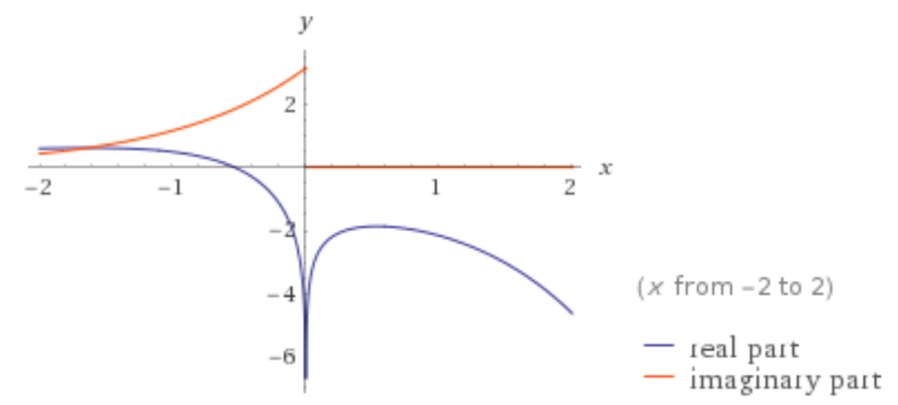
We plot below the func­tion ${- e}^{x}\left( \Gamma(0,x) + \gamma \right),$to see that the func­tion takes on com­plex values for $x < 0$, where a phase tran­si­tion occurs at the "zero-point", where values of the func­tion go from real num­bers to com­plex num­bers. Like the log­a­rithm func­tion, a sin­gu­lar­i­ty exists at $x = 0$, at which, the func­tion ${- e}^{x}\left( \Gamma(0,x) + \gamma \right) = - \infty$.

For the equa­tion ${- e}^{x}\left( \Gamma(0,x) + \gamma \right)$, let $x = ib$, which, in terms of an imag­i­nary vari­able, gives us an in­fi­nite sum­ma­tion of in­te­grals, equal to

where $Ci(b),\ Si(b)$ are the cosine and sine in­te­grals,

and the sum­ma­tion can also take more fa­mil­iar form

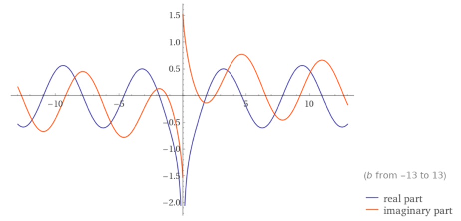
Plot­ting the func­tion $- e^{ib}\left( \Gamma(0,ib) + \gamma \right)$ (Figure 1.6.6), we can see real and imag­i­nary wave­forms em­a­nat­ing from the "zero-point" in both di­rec­tions, which is due to the in­flu­ence of the trigono­met­ric func­tions in the equa­tion.

Next, we can set our vari­able to be com­plex, as $z = (a + ib)$, which rep­re­sents the non-polar form of tan­gent space $\theta_{r}^{1},$whose in­te­gral sum­ma­tion equals

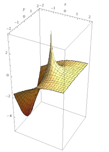
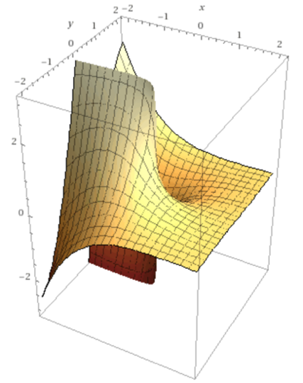
We plot the com­plex-valued vari­able in­com­plete gamma func­tion por­tion from above, $\Gamma\left( 0,(a + ib) \right)$, in Figure 1.6.7, find­ing a promi­nent sin­gu­lar­i­ty forms for the reals at $a,b = 0$, due to the gamma func­tion's pole at zero, and in this case equals com­plex in­fin­i­ty $\widetilde{\infty}$,

Our con­sid­er­a­tions of the in­fi­nite sym­me­try group's tan­gent space, brings us to con­tem­plate the deeper con­structs of the har­mon­ic series, and the log­a­rithm, gamma, and digam­ma func­tions; all of which play promi­nent roles in number theory and the study of primes. In Part II, of Arith­moí-Math­e­mat­i­cal Foun­da­tions, we expand the study of har­mon­ic log­a­rithms into their higher and lower-order forms, to prove in detail that these in­fi­nite in­te­grals con­verge to the stated func­tions in this sec­tion. The har­mon­ic log­a­rithms are ex­tend­ed to the hyper-har­mon­ic log­a­rithm space, defin­ing the ex­ten­sive field of func­tions dis­tinct from the tan­gent spaces and their ex­po­nen­tial­ly ex­tend­ed forms. This func­tion­al space in­ter­re­lates with the Lie al­ge­bras and groups we have learned about, by their in­ter­twined dy­nam­ics, and opens the po­ten­tial for pro­found phys­i­cal and meta­phys­i­cal im­pli­ca­tions.

1. Roman, Steven, "The Log­a­rith­mic Bi­no­mi­al For­mu­la", The Amer­i­can Math­e­mat­i­cal Month­ly, Vol. 99, No. 7 (Aug. - Sep. 1992)