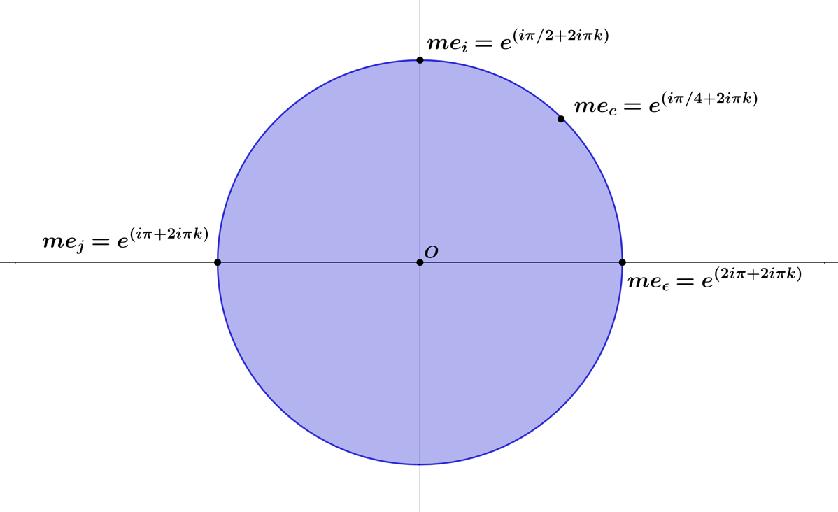
Previously in this book, we introduced Cayley's theorem, which states that for a group , there is a symmetric group that acts on , and is then isomorphic to a subgroup of the symmetric group. In the last section, the minimal element, , was used in the expression to count the number of Lie algebra generators a particular group had. This section will show geometrically how Cayley's theorem relates to the minimal element. First, we define the first four minimal elements as points on the complex unit circle, seen in the figure below, and as follows
(1.7.1)
Figure 1.7.1 – Minimal elements on the complex unit circle
On the unit circle, the minimal element, , represents the identity set
(1.7.2)
having one sole Lie algebra generator. By rotating radians on the unit circle in either the positive or negative direction, we arrive at , which as the set of permutations, , now contains two Lie algebra generators
(1.7.3)
which is inclusive of the identity element representing . If we define the identity group , containing the permutation set , and the split complex group , with the permutation set , it holds that
(1.7.4)
Since the permutation set for the group is on the unit circle, we can define the group as
(1.7.5)
and likewise, the group , can be defined as
(1.7.6)
Given that is defined by its element in the set , and , and both sets are in the set
(1.7.7)
it is also true that the is a subgroup of
(1.7.8)
can be seen as the next-ordered symmetry of the unit circle, which is consistent with Cayley's theorem, being that the group is a subgroup of the symmetry group , based on the minimal element of choice
We can also consider the next-ordered symmetry set, , as the unions
(1.7.9)
which represents the fact contains its minimal element, and its subgroup set
We arrive at our next minimal element, , by rotating radians in the positive direction from . The symmetry of the complex unit circle becomes apparent, given that we could choose to rotate instead by radians in the negative direction to arrive at . We know the circle's symmetry, and this symmetry also applies to the minimal element. This is an important concept, and it is related to the ontological concept of net-zero. Analogous to the cyclic group, which defines a group containing at least one Lie algebra generator capable of generating all elements in the set, the positive and negative minimal elements, , are Lie algebra generators, both of which can generate all the elements in the set, shown for both cases as
(1.7.10)
Nested in these two examples is the symmetry of the next lower order generator set, which is represented by the symmetries
(1.7.11)
which are the Lie generators on coinciding with the generators of the set. By stating it in these terms
(1.7.12)
subgroup nesting of the minimal element sets is apparent when considering the exponents.
Next, the minimal element represents a rotation in the positive direction of radians from the identity
(1.7.13)
whose counterpart rotation in the negative direction, , is
(1.7.14)
Like and , we will define the positive and negative-valued as
(1.7.15)
the variable choice of defines these as cone numbers but also light, which we will consider later in the chapter. As was the case for , both Lie algebra generators , generate all the set's elements
(1.7.16)
and
(1.7.17)
The nested minimal element symmetry equivalences for are
(1.7.18)
where the even exponent pattern that has emerged is due to our choice of subsequent minimal elements that are half the previous one. Our selection of minimal elements has led to the symmetric division of the complex unit circle into smaller and smaller portions. The nested minimal element symmetry equivalences have exponents related by multiples of the prime number . This prime number relationship relates to our initial manner of sectioning the complex unit circle, a symmetric halving of successive sections, which represents taking successive square roots of the group
(1.7.19)
Accordingly, the inverse of the above process of these successive square roots is taking the square of a minimal element, which results in the adjacent minimal element of a lower order, seen as follows
(1.7.20)
The number is the only even prime number, and it is related to the exponent values for the sectioning as an ever-increasing set of minimal elements, which is based on the sectioning ratio , and the iteration, which runs from , of the minimal element
(1.7.21)
and we note for any , we have
(1.7.22)
In the expression above, all the exponent values for the sectioning of in the set are built upon the reciprocal compositions of the prime number . The minimal element with , is equal to the composition
(1.7.23)
which has the integer prime number composition counterpart
(1.7.24)
This leads us to see that all minimal elements, of the group are related to the reciprocal prime number , and its exponential composition, except the sectioning identity , which is analogous to the integer number . The reciprocal prime number , should also be considered the second element in the harmonic series, and the identity as the first in the series, .
Considering the first prime number, , we move on to the next prime number, , and section into three parts, where the set of elements, , is based on the successive powers of minimal element
(1.7.25)
around one rotation of the complex unit circle. Each power of the minimal element , is explicitly
(1.7.26)
and like previous examples, the directional choice of rotation away from the identity yields a minimal element, which can generate all Lie algebras in the set. We should also note that also generates all elements of the set , given that
(1.7.27)
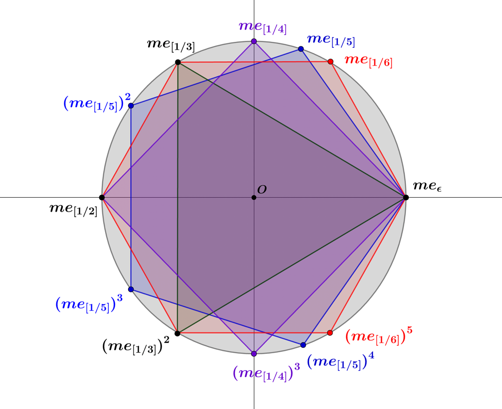
We continue the process for the following three minimal element sets, which represent the reciprocal numbers and along with the set , we plot each below as a polygon inscribed in the complex unit circle, where the polygon vertices represent the positively oriented path the minimal element takes around the unit circle. The number of vertices is equivalent to the respective numbers .
Figure 1.7.2 –Prime and non-prime minimal element sets as polygons on the complex unit circle:
Each polygon in the figure above shares the same identity minimal element, , which is analogous to how every integer has the number as a common factor. The first six integers contain the identity integer, , three prime numbers, , and two composite numbers, . The numbers and result from the following prime number products
(1.7.28)
which can be further classified as even composite numbers. All even composite numbers will be composed of at least one factor of the number , the only even prime number. The polygons that represent the even composite numbers and have vertices at points on the unit circle, which their composing prime numbers have already passed through. For instance, the set , represents the composite number 4, and shares a vertex with the prime number -related set , at the point . The set , representing the composite number , shares vertices with the prime number -related set at the points and a vertex with its other prime number related set at These shared vertices represent composite numbers' beautiful geometric relationship with their prime number generators in the complex space of the group.
The distribution of prime numbers is highest in the range of the lower-valued natural numbers. In the set of numbers from to , there are prime numbers, even composite numbers, and odd composite numbers, the first of which is the number 9.
The radian measures for the vertices of the first thirteen polygons are shown in the table below, representing both the element of the harmonic series and the reciprocal integer, where each -gon has a total of vertices, numbered to .
Table 1.7.1 – Vertices of polygons-in arclength from. Red values are primenumber vertices, and blue values are repeating compound vertices.
In the table, repeating prime number vertices are symmetrically distributed about the real-axis for each polygon, where, for example the set for the -gon is
(1.7.29)
where the set starts at the identity, then passes through two novel vertices, the first vertex for the geometric prime number , two more novel vertices, the second vertex for the prime number , and finally, the last two novel vertices. These novel vertices will repeat starting with the -gon, and this can be seen best by following the integer progression for , where starting at the prime number , all its elements repeat in -gon, and all its elements will then repeat in the -gons. The reason for this is straightforward since it is related to repeating prime numbers of the same value in composite numbers, seen by considering the prime number generators for each of the polygons
(1.7.30)
where represents the prime number. We see above that the numbers and are compound numbers composed solely of the prime number , while the number is a compound number composed of two prime numbers . All prime number vertices can be expressed as
(1.7.31)
where is the prime number, with an integer value , and except for the prime number , is a rational that is always over odd prime
(1.7.32)
making them irreducible. This differs from the integer numbers, , which will have vertices in two forms
(1.7.33)
(1.7.34)
based on whether is an odd or even integer. Except for the number , when is even, we immediately know it is a compound number, given it will contain reducible rational numbers in its set of vertices. The integers will be prime numbers if all the vertices of its inscribed -gon representation in the unit circle are irreducible. Importantly, this enables us to geometrically see how prime numbers differ from compound numbers since a prime number , will not possess internal symmetries allowing any lower integer-valued prime polygon less than, to rotate in a vertex-to-vertex fashion in the complex unit circle.
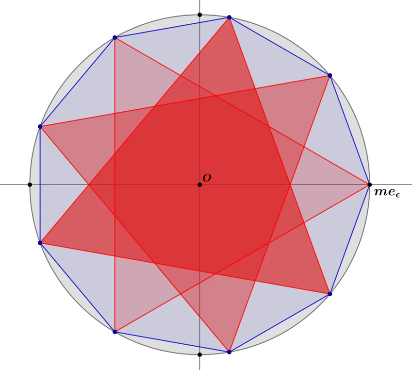
To show this geometric characteristic of the prime numbers, in the following figure we graph the inscribed -gon representing the set of vertices with a minimal element basis of
(1.7.35)
and its geometric prime number generator, the equilateral triangle, -gon, with a minimal element basis of
(1.7.36)
Figure 1.7.3 – The inscribed -gon representing the integer ,and the
three distinct orientations of its prime number generator.
We see the equilateral triangle has three unique orientations in the -gon, which is the geometric result of the number 's composition
(1.7.37)
We now have a better geometric sense of how prime numbers can be expressed in complex space, leading us to formally define the geometric primes.
Definition (1.7.38) - The Geometric Primes,, are the geometric representation of the prime numbersas inscribed regular polygons in the complex unit circle, withvertices,, symmetrically arranged around the complex unit circle,, by distance intervals equal to the minimal element basis, forming the set of verticesdefined as
and these vertices have unique location values for all geometric integers less than, and are unique to any geometric prime in the set of all geometric primes.
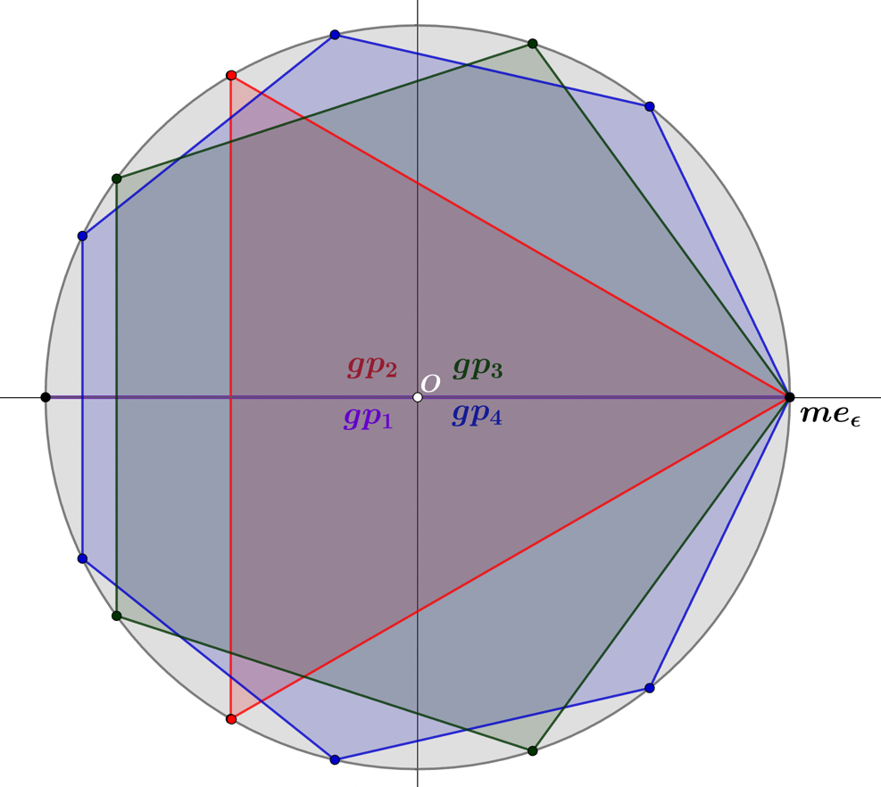
Figure 1.7.4 – The geometric prime numbers ,
inscribed in the complex unit circle, representing regular polygons.
Plotted above are the polygonal representations of the first four geometric primes, g, where the number of vertices coincides with the prime number's integer value. All vertices have unique location values compared to all integers of lower value, including geometric primes and geometric composites. The vertex location values of all geometric primes continue to be unique compared to other geometric primes in the set of all geometric primes. Composite numbers will share vertex values with geometric primes, given that these numbers are composed of prime number products.
Theorem (1.7.39) – Except for the identity vertex, all vertices of the geometric prime,, for, can generate all vertices of its inscribed regular-gon.
Proof – By definition, the first vertex is located a distance in radians offrom the identity vertex
The set of positively and negatively oriented vertices on the boundary of the complex unit circle, with the minimal element basis, is the set
for which each vertex is symmetrically spaced around the boundary of the unit circleby an arclength distance,
Given thateach vertex will be located at an arclength distance from the identity atof
for integer values ofthrough. Therefore, the numerator remains, the denominator isfor, and irreducible given it is prime. The set generated by a vertex located atis
which is equivalent to the set
As the set of verticesis on the complex unit circle and defined as modulo, the set is equivalent t
which can be stated as
given that
This proof shows that the geometric primes represent cyclic groups by the criteria that all vertex elements, except for the identity vertex, can generate all vertex elements.
The prime numbers are intimately connected to harmonic series and the Riemann zeta function, for , evidenced by the Euler product formula
(1.7.40)
which was proved by Euler and published in To show how Euler arrived at his result, we take the following two related zeta function infinite series representations
(1.7.41)
and subtract the second series from the first
(1.7.42)
Next, we take the series
(1.7.43)
and subtract this from to find
(1.7.44)
and this is a series with all reciprocal prime number factors of and removed. The process repeats infinitely, resulting in
(1.7.45)
and dividing both sides by the infinite product of with terms of the form , we find that
(1.7.46)
For , the zeta function, simply reduces to the harmonic series
(1.7.47)
and the Euler product is
(1.7.48)
To show how the Euler product relates to geometric primes, we first look at the following contour integral
(1.7.49)
We consider the unit circle by setting to find , and the integral above becomes
(1.7.50)
Simplifying and evaluating the integral, we find the result
(1.7.51)
which is consistent with the perimeter distance of the complex unit circle in radians. The minimal element represents the first vertex of each -gon located in the counterclockwise direction from the identity vertex. The perimeter distance of this vertex is
(1.7.52)
where is the reciprocal integer value and is the element of the harmonic series. We can express the zeta function as a product with the previous contour integral as
(1.7.53)
which is equivalent to
(1.7.54)
where the Euler product holds for the harmonic series terms in parenthesis, and we can express the zeta function as a product with the contour integral of the complex unit circle
(1.7.55)
In the last chapter, we considered the series of the natural numbers as the element-to-element inverse of the harmonic series. The triangular numbers, , are defined as the sums of successive sequences of the natural numbers to , as follows
(1.7.56)
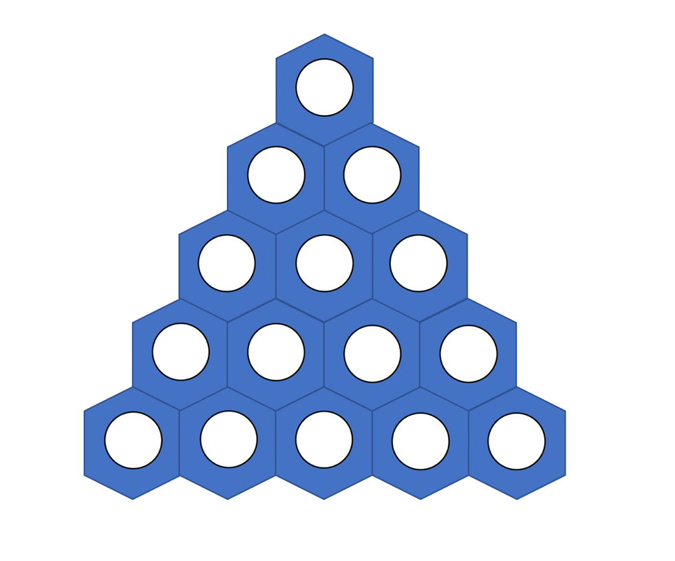
These numbers are triangular since they count objects arranged in the equilateral triangle, with one element in each row/column position. For example, the fifth triangular number is seen in the figure below, where results from counting all the white circles from each row.
Figure 1.7.5 – The triangular number and its relationship to the equilateral triangle.
Evaluating the first five triangular numbers, each representing a successive sum of rows from the equilateral triangle from the figure, we find
(1.7.57)
Next, we consider how the number relates to its respective sum, by evaluating the ratio for each row, as follows
(1.7.58)
finding the distinct pattern that each ratio increases by compared to This ratio generalizes as the expression
(1.7.59)
whereby solving for , we find the triangular numbers have the closed form
(1.7.60)
Given that a binomial coefficient is defined as a ratio of factorials
(1.7.61)
the numerator of , can also be expressed as a ratio of factorials
(1.7.62)
which leads to the binomial coefficient expression
(1.7.63)
and the triangular numbers can be defined as
(1.7.64)
As we found previously, the radian distance for each vertex of the inscribed polygon representation in the unit circle can be expressed as the minimal element relationship
(1.7.65)
and by taking the principal valued logarithm for each element in the set above, we can define the set , to represent the set of radian distance values from , for each vertex of the polygon, as
(1.7.66)
Next, we choose to find the total vertex distance, but summing each distance element in the set , to find the series
(1.7.67)
for which we factor out
(1.7.68)
and find the presence of the triangular numbers in the series. We can now substitute our closed form for the triangular numbers into the series
(1.7.69)
finding that our total vertex distance also has a closed form as follows
(1.7.70)
Next, we solve the series by equating the triangular numbers to their factorial ratio equality, as follows
(1.7.71)
and likewise, we find the total vertex distance summation relates to the binomial coefficient
(1.7.72)
We return to the set , which represents the exponential form for each vertex location on the complex unit circle
(1.7.73)
which is equivalent to the form
(1.7.74)
The following exponential product sum
(1.7.75)
is analogous to the total vertex distance summation, and specifically, they are the following logarithm and exponential relationships
(1.7.76)
and
(1.7.77)
which shows the connection these products and sums have with the minimal element Lie algebra. As expected, the result of the product sum has the exponential form
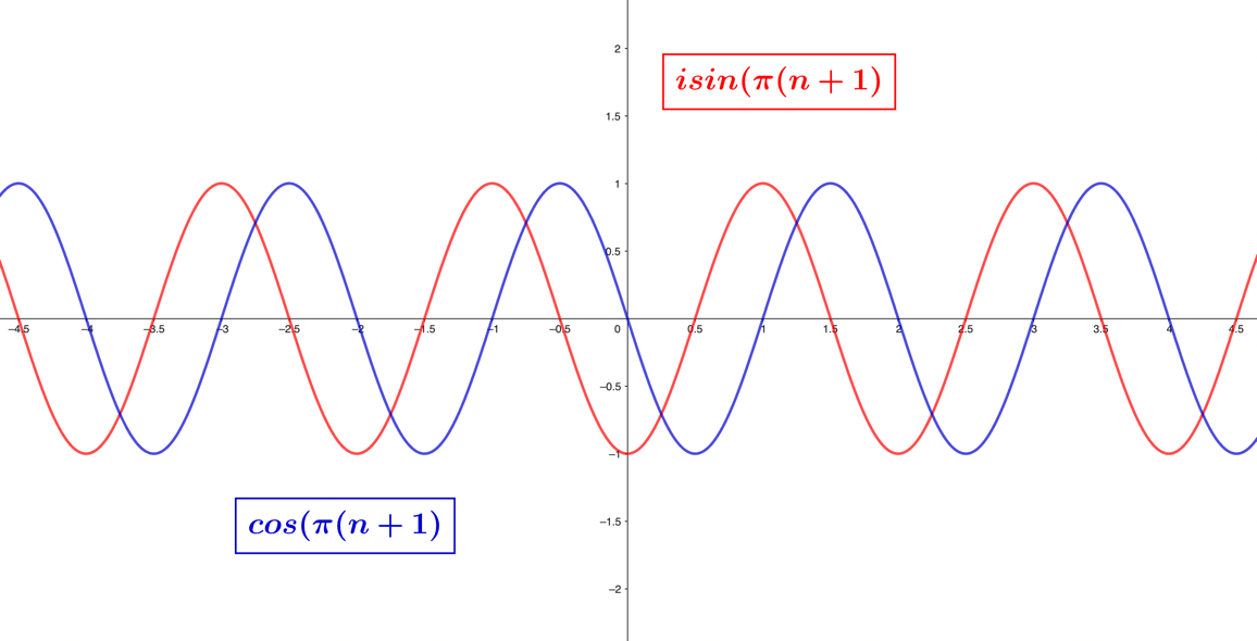
(1.7.78)
which for integer values of , the value will oscillate between for even and for odd. Suppose we extend the variable from the natural numbers to the reals, . For this case, we plot the function in the figure below, finding the familiar waveforms of the exponential function, which are phase-shifted by radians.
Figure 1.7.6 – The product sum plot:
As we continue studying the singularity by probing deeper into it mathematically, the importance of triangular numbers becomes more apparent. The exact way they are related to the elements of the harmonic series is easy to see by starting with the previously derived result
(1.7.79)
which we solve for , to find the inverse relationship it has with the triangular numbers
(1.7.80)
which leads to the summation expression for the harmonic number as
(1.7.81)
To show the beauty these numbers have, we consider the summation of the inverse triangular numbers,
(1.7.82)
which we see is a series composed of increasing subseries of rational numbers. To see if this series converges, we take each element in the series
(1.7.83)
then take the partial fraction decomposition of this result to find
(1.7.84)
which we can now sum individually to find
(1.7.85)
Both sums are related to the harmonic numbers, and given that
(1.7.86)
(1.7.87)
we can see that this series converges to
(1.7.88)
which can be simplified as follows
(1.7.89)
and therefore, we have that
(1.7.90)
A beautiful thing about these numbers is that when the sum of the numbers is evaluated as , we find it converges to 2
(1.7.91)
Intuitively, we can see this convergence result by first looking at the set of successive values of ,
(1.7.92)
and after factoring out the number we find
(1.7.93)
where the values in the set approach the value of , as the values of get larger. An evident relationship exists between this and the harmonic series, seen when expressing the set as
(1.7.94)
where each element is now represented as a difference of and the ordered elements of the harmonic series. This relationship yields the following partial sums of numbers, and how they relate to the harmonic numbers as
(1.7.95)
where we arrived at this expression by first considering as the series
(1.7.96)
which, when expanded, is found to be a telescoping series
(1.7.97)
Therefore, the partial sum of is
(1.7.98)
and after rearranging the expression by solving for , we find
(1.7.99)
which simplifies to
(1.7.100)
and by decreasing the iteration for the harmonic numbers by one, this yields the following expression for
(1.7.101)
As we described previously in the section, the harmonic series is related to the prime numbers by way of the Euler product
(1.7.102)
which in the case when , the Riemann zeta function is related to the primes as the following equivalence
(1.7.103)
Our defined numbers are related to the tetrahedral numbers, which are defined as the summation of the triangular numbers to
(1.7.104)
with the difference being in the case of , we are summing the inverse values of the triangular numbers,
Our work showing the relationship between the inverse triangular number sums , the harmonic series, and the harmonic numbers, , lets us learn precisely how the inverse triangular number sums are related to both the Riemann zeta function and the prime numbers. To start, since the harmonic number is equal to
(1.7.105)
as , the following limit is equal to the zeta function, for
(1.7.106)
and based on our equality, both of the following limits are equal to
(1.7.107)
Taking the expression found previously for ,
(1.7.108)
and with simple algebraic manipulation, we find
(1.7.109)
and given that
(1.7.110)
it is also true that
(1.7.111)
This leads to the identity
(1.7.112)
where we note that
(1.7.113)
Using this identity, we expand the limit involving the inverse triangular number summation
(1.7.114)
and equate it to the function , to find
(1.7.115)
In the expression above, the is offset term-by-term by the ones in the bracketed terms, while the other limit is equal to one
(1.7.116)
given that
(1.7.117)
which once again verifies that
(1.7.118)
Therefore, is equal to the following series of terms
(1.7.119)
With the expression above, we see the numbers are related to the function by way of well-behaved infinity minus the infinite series of the numbers. To further consider a more exact relationship between the zeta function and the numbers, we must first define the Tau function .
Definition (1.7.120)– The Tau function, for, represents the infinite series of the following inverse triangular numbers
for, defined as
and as a series, is the element-by-element additive inverse of the respective zeta function
It is easy to see the additive inverse property the function has with the zeta function, given that
(1.7.121)
and we will denote the infinity that results from the sum as
(1.7.122)
Geometrically, the numbers of the function travel in the oppositive direction in the complex plane compared to the series of numbers from the function. Specifically, the numbers are related as opposite-valued Euler products
(1.7.123)
which we prove for in the theorem that follows.
Theorem (1.7.124) – The following Euler Productdefines the Tau function
Proof – The functionis defined, for, as the following summation
which, when expanded, is equivalent to
this arranges to
whererepresents the infinite sum of identities
We proceed to calculateby algebraic manipulation of the series, where we calculate first
and subtract this from
where all even-valued reciprocals have canceled, and the above simplifies to
We continue this process for the subsequent two iterations as follows
where all successive compound reciprocals for the prime reciprocalsandhave also been eliminated from the right-hand side. By extending this process infinitely, the result is
for which, factoring and simplification yields
and after dividing both sides by the infinite reciprocal prime-related product series, we find
which equals the stated theorem
Previously, we arrived at the equality for
(1.7.125)
After substituting our defined and the function, the expression is equal to
(1.7.126)
and solving for , we find the following additive inverse equality
(1.7.127)
which is consistent with the additive inverse properties in the definition for This equality, along with the specific solution to our previous proof
(1.7.128)
present the means to understand the infinity of ones mathematically. Specifically, how it splits into the elements of the harmonic series with the element-by-element additive inverse series of inverse triangular numbers. We can also define a very concise equality for the identity by solving for in the following expression from our proof
(1.7.129)
where the difference between products of two distinct infinite series with the infinite product of reciprocal primes yields the identity. Given that
(1.7.130)
this is also equivalent to our identity expression
(1.7.131)
and once again, mathematics never fails to impress with its beauty and cohesiveness.
We turn to prime numbers and their representations in group theory. This book has focused on the prime number , from the standpoint of groups, and the geometric prime is encapsulated in matrix algebra as the set , composed of the following two generators
(1.7.132)
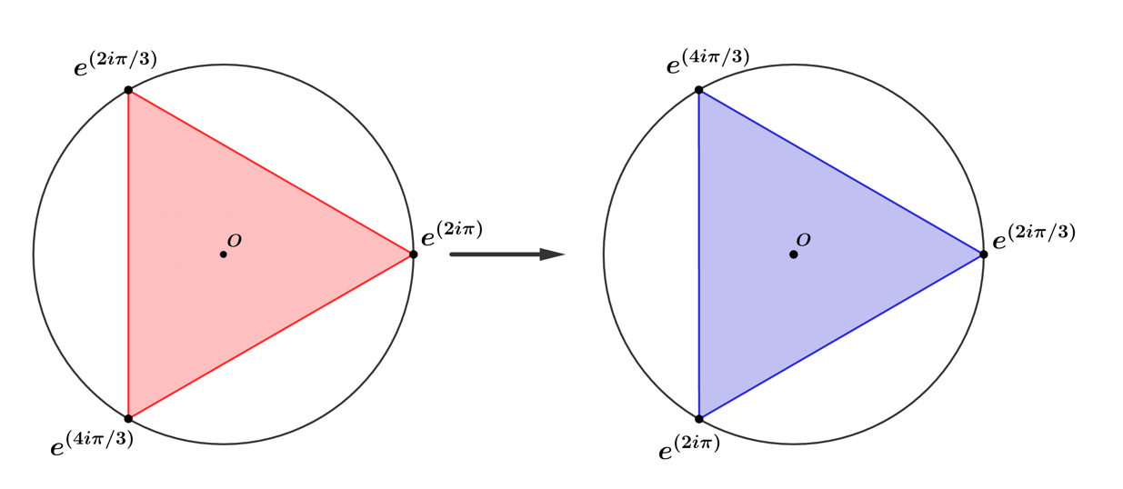
The matrices are the same generators from our group theory study but differ regarding their direction of rotation when acting on a position vector. To show this mathematically, we define a vector , which represents the three vertices of the inscribed geometric prime arranged in counterclockwise order from left to right, and take the following matrix-vector product
(1.7.133)
which represents a clockwise rotation of the vertices by radians, shown in the figure below.
Figure 1.7.7 –Clockwise rotational transform of , by matrix product. A red triangle represents the initial coordinates of vertices, and a blue triangle shows the final coordinates of vertices.
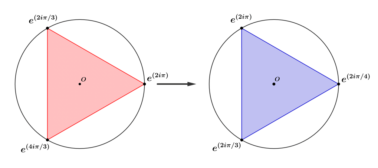
As stated, we find that the matrix-vector product , rotates the plane in the opposite direction, counterclockwise, given that
(1.7.134)
whose transform we show in the figure below.
Figure 1.7.8 –Counterclockwise rotational transform of complex plane, by matrix product, the red triangle represents the initial coordinate locations of vertices, blue triangle shows the final vertex coordinates.
We direct the reader's attention to the matrix below
(1.7.135)
where is just a dummy variable, and like the prime number , the matrix cannot be split equally into smaller submatrices, except for sizes and itself, . We compare this to the composite geometry of the integer nine, which has a square matrix representation, but we can divide the matrix into nine even sections
(1.7.136)
which underscores the fact it is composed of matrices, and this sectioning of the matrix is the only way to do so. Compare this to the composite geometry of the integer , which has two unique ways to evenly section its matrix
(1.7.137)
(1.7.138)
where the first represents a sectioning of matrices, and the second a sectioning of matrices, signifying is composed of the geometric prime numbers and .
For the geometric prime set
(1.7.139)
we now return to the anti-diagonal symmetry of the Cartan algebra discussion in Section 1.2.9, where each Lie algebra generator in the set has symmetry about the anti-diagonal axis. The identity matrix represents the diagonal axis, and, when taken as a product with another matrix, acts to scale the values of that matrix's entries. The anti-identity matrix can be thought of as the analog of the relationship the identity matrix has with the diagonal, and this anti-identity matrix we will define as
(1.7.140)
which is the same as the -type Lie algebra that we have defined previously. Similarly, we can define that
(1.7.141)
which we arrive at by rotating the and Lie algebras by 90 degrees in the clockwise direction, and the reader should consider these transforms as higher-dimensional rotations of the geometric prime. From the standpoint of matrix representation theory, these dimensional transforms are the result of the product of the rotation matrix , with the elements of the set , seen as follows
(1.7.142)
It is important to note that any of the -type matrices can generate the same matrix-matrix products above, and our choice to use the anti-identity matrix, , has its basis in maintaining consistency.
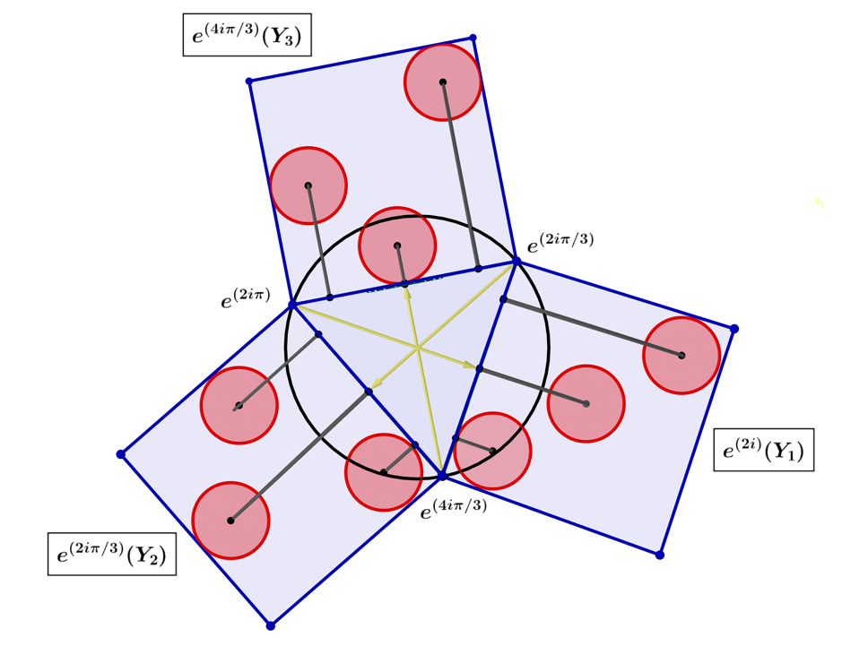
To better understand the higher-dimensional rotations of the geometric prime algebras, we show in the figure below the arrangement of the algebras along the edges of the equilateral triangle, where each algebra is positioned on the edge coinciding with its vertex symmetry (yellow arrows). Additionally, the elements of the algebras are represented as red circles, instead of s, in each of the squares.
Figure 1.7.9 – The geometric prime algebras arranged on the edges of each algebra's vertex symmetry.
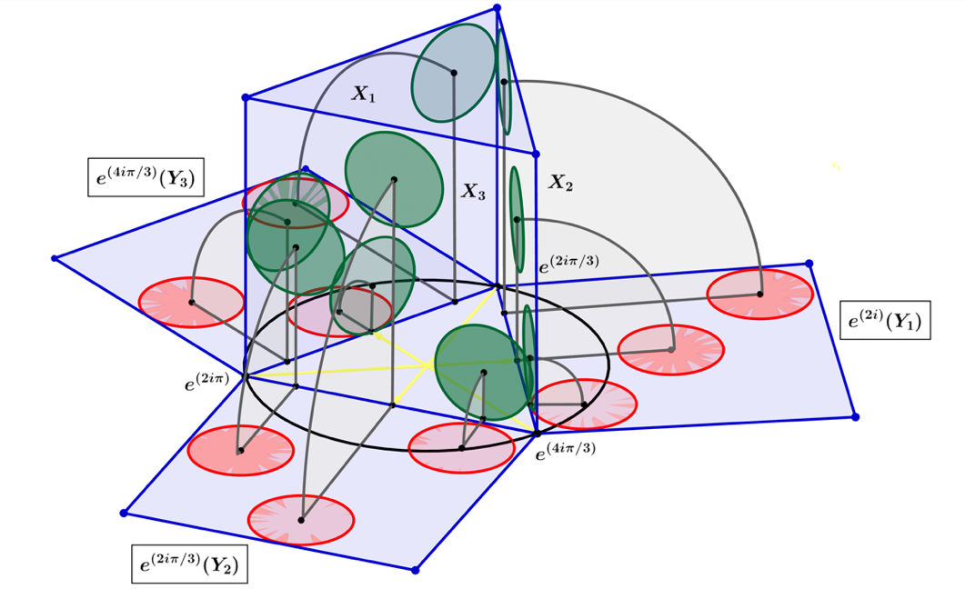
Figure 1.7.10 – The geometric prime set rotation , squares containing the red circles represent the geometric prime algebras and the squares with green circles represent the set of algebras .
Next, we look at the set of Lie algebra generator rotations in matrix form as
(1.7.143)
and consider the extension of the geometric prime, into the higher-dimensional space, which is presented in Figure 1.7.10. We can see in the figure that each algebra projects into the higher dimension of its specific algebra, which is onto a face of the triangular prism rising from the geometric prime's equilateral triangle.
Just as the prime numbers are the building blocks for the integers, the geometric primes are the sine qua non of the Lie algebras we have studied. In the higher-dimensional complex spaces, the geometric primes are the building blocks of the composite -gons. Still, we will find they are responsible for building the algebra's dimensions, and we will touch upon this subject in the next section.
We return to the inverse triangular number set
(1.7.144)
to further consider how it is related to the minimal element, , which we recall is defined as
(1.7.145)
When assuming a positive-valued , the first vertex of the representative -gon will be oriented at a counter-clockwise distance of radians from the identity. We take the set and consider its values to be on the complex unit circle and in radians, where is equal to
(1.7.146)
and the set would then equal
(1.7.147)
Each value in the represents the first vertex of the representative -gon from the identity in the clockwise orientation and represents the argument that defines the negative-valued minimal element, . In the case of the geometric prime, is equal to
(1.7.148)
which has the equivalent form with a positively valued argument
(1.7.149)
By considering the inverse triangular sum , we find it equals the same argument above, given that
(1.7.150)
and the same is true for all elements in the set where the negative-valued minimal element, , is equal to
(1.7.151)
Going back to the Euler product we described,
(1.7.152)
where the contour integral , we know is equal to , it becomes clear that the terms containing the reciprocal primes are equal to the reciprocal primes of the set , which we define as
(1.7.153)
and this set also represents the radian distance of the negative minimal element , for reciprocal prime values, defined as
(1.7.154)
Similarly, the positive-valued minimal elements with reciprocal prime values, are defined as
(1.7.155)
and elements between the sets with like reciprocal prime number basis are related as conjugate pairs, where their products are equal to the identity
(1.7.156)
For any -gon inscribed in the complex unit circle, the value is the sum of conjugate product pairs, given that
(1.7.157)
and the partial sum of is simply equal to
(1.7.158)
We now have a geometric interpretation of the prime numbers, representing a solid foundation we will build upon in the next book in the Arithmoí series. In this section, we have found several connections prime numbers have with group theory, higher dimensional complex spaces, and the triangular numbers, made possible by putting the minimal element into its proper perspective.