In this final section, we explore the geometry of matrix group conics through visualization. The reader is most likely familiar with the Cartesian representation of the unit circle , and this relates the invariant unit distance from the origin to the coordinates , which together, form the equation of a circle. In the 2-dimensional matrix form, the determinant of the unit circle's polar representation gives us the trigonometric determinant form
(1.4.177)
and comparing this to the Cartesian form, we see that and . In more general terms, we can state the Cartesian form and how it relates to its radius , as
(1.4.178)
and in the polar form
(1.4.179)
A similar Cartesian-to-polar form exists for hyperbolic geometry, where we start by taking the determinant of the matrix representing the unit hyperbola
(1.4.180)
which in Cartesian coordinates translates, as , having the determinant
(1.4.181)
The unit hyperbolic representations also present with invariant unit length for their matrix determinants, which is typically denoted as a radial distance from the origin in the hyperbolic trigonometric representation
(1.4.182)
which, in Cartesian form, is expressed as
(1.4.183)
The cone is classically represented by lines in real Euclidean space, while the representation for our matrix groups will be more detailed. We recall the two-dimensional matrix group representation for the cone number
(1.4.184)
which has the determinant
(1.4.185)
Here, we also see the invariant unit length, by way of the unit-valued determinantsIt may not be obvious in the form above, but this cone matrix group is a balanced representation of the unit circle and the unit hyperbola. Considering the complex coordinates our cone group example represents the exponential function , where it becomes apparent that it is equal parts real exponent and imaginary exponent, evidenced by rewriting the exponential, as
(1.4.186)
Now, we can represent this as the product of two matrix groups
(1.4.187)
and when considering the determinants of these matrix groups, we find
(1.4.188)
which is equivalent to
(1.4.189)
In the determinant products above, the angle is downscaled by the factor when compared to the individual unit circle and hyperbola, making iterative circular rotations for each , We are tempted to consider the relationship above in terms of their Cartesian forms, representative of the unit hyperbola and unit circle
(1.4.190)
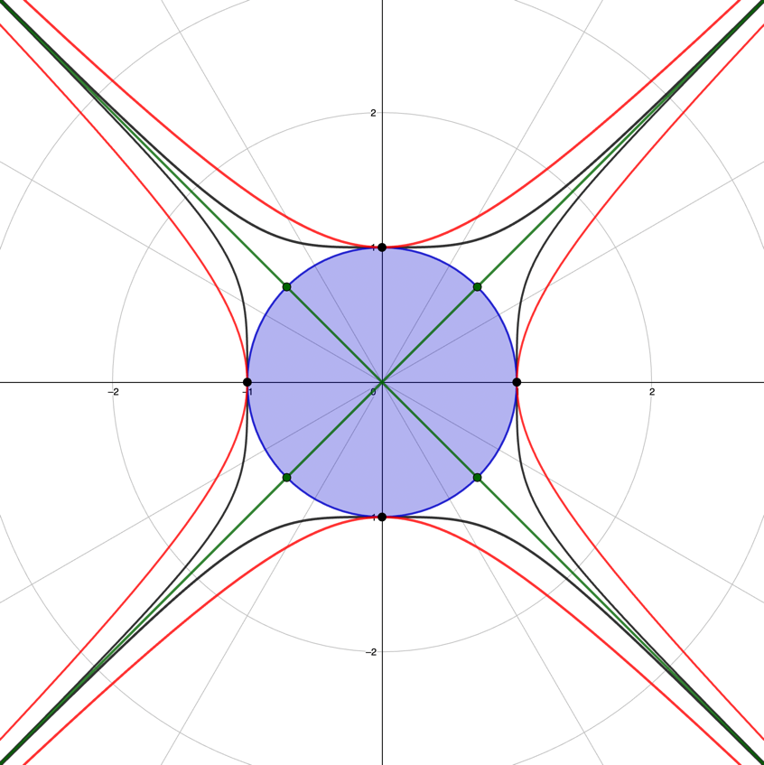
This Cartesian form does work to give us the first glimpse at what the product of a hyperbola and circle might look like when compared to the standalone forms of the unit hyperbola and circle (Figure 1.4.21).
Figure 1.4.21 – A two-dimensional slice through the -plane of a complex conic section.
In the graphical representation of the equation , the unit cone does take on the appearance of the asymptotes of the unit hyperbola, seen as it extends further from the boundary of the unit disc. Shown in the image, is the unit hyperbolae (red), the unit cone's curves/asymptotes (black), the unit circle (blue), and the hyperbolic asymptotes (green).
To ensure the Cartesian cone numbers are mathematically consistent, we begin with the original product of the matrices
(1.4.191)
to express these by the following product of matrix exponentials
(1.4.192)
Taking the determinant of the resultant matrix above,
(1.4.193)
to then consider this result in the Cartesian form of the unit hyperbola raised to the power
(1.4.194)
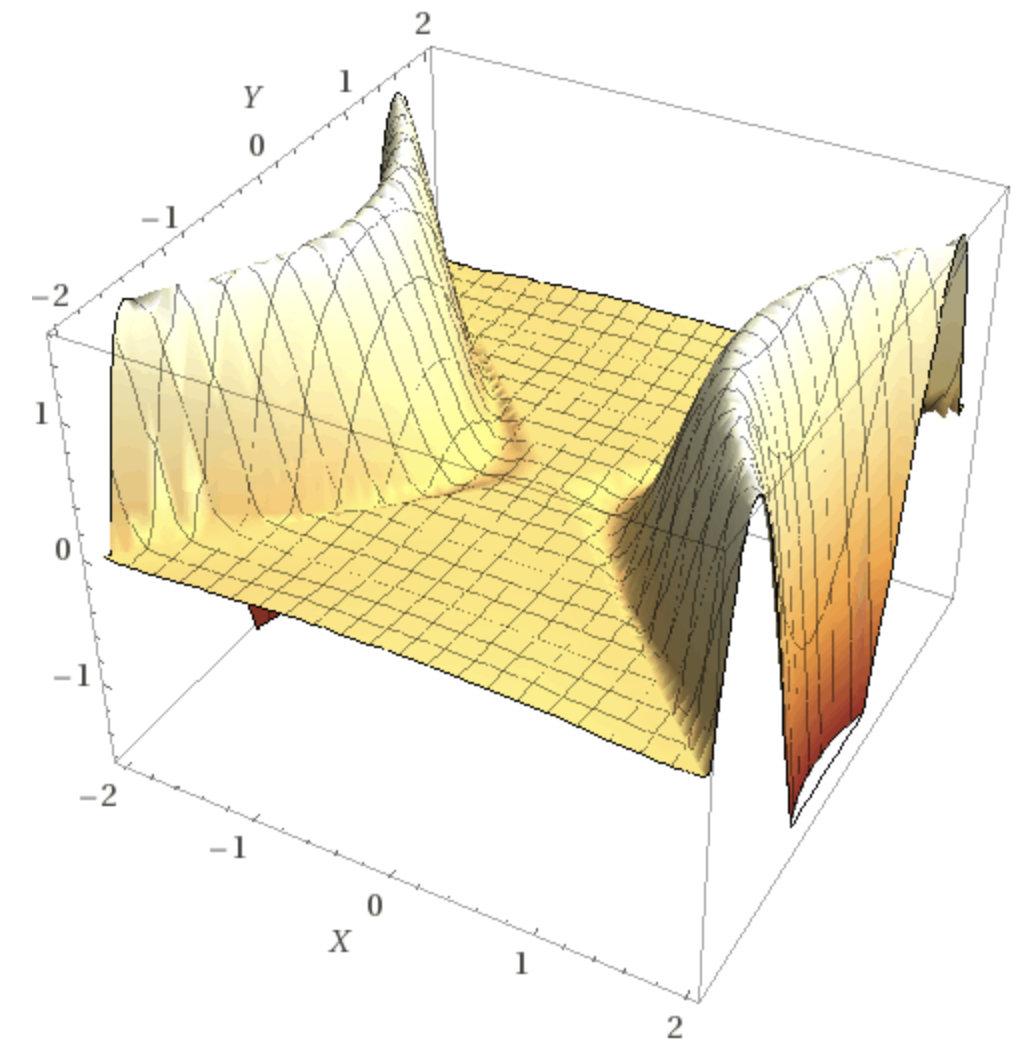
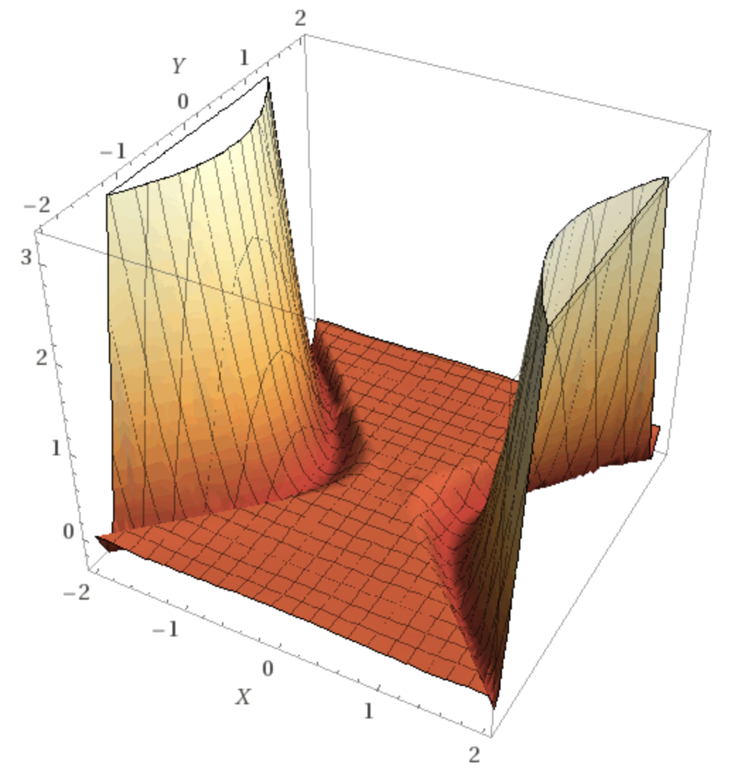
Figure 1.4.22 – 3D plots of the equation, real part (left) and imaginary part (right).
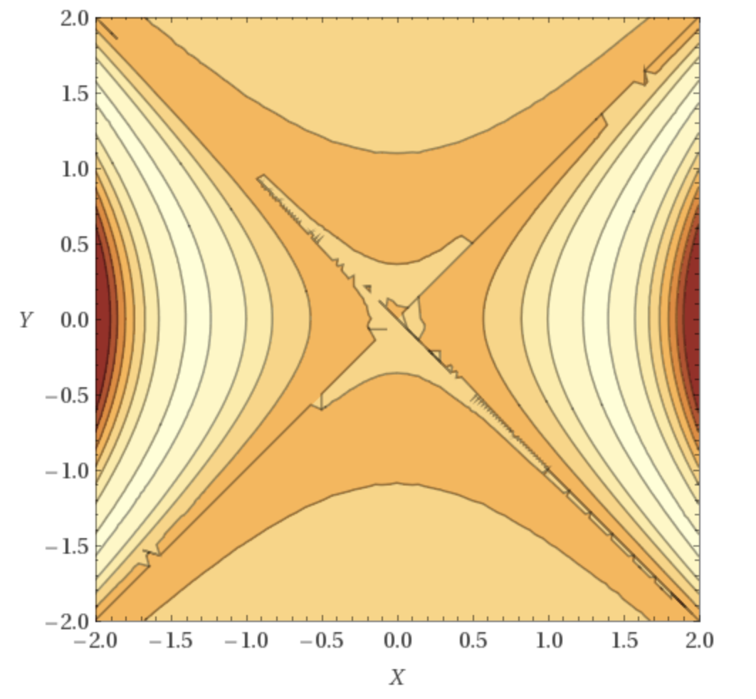
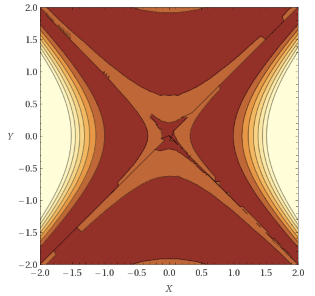
To gain an intuition for what this function looks like, we plot the imaginary and real portions in three-dimensions in Figure 1.4.22, and as contour plots in Figure 1.4.23.
We can see a cone structure that emerges in the real and imaginary-valued three-dimensional/contour plots. Turning to the cone elements of the symmetry group, we start by taking a tangent space element , like that we worked with for the subgroup, and define , as
(1.4.195)
The next step is to consider how to arrive at the entire tangent space for the -oriented double cone. To do this, we will have to rotate the matrix in the -plane, by using as the axis, which is exactly what the -element does! Denoting the exponentiated -type element , as and using the angle argument , we have
Figure 1.4.23 – Contour plots for the equation real part (left) and imaginary part (right).
(1.4.196)
The product,, for , the angle argument of , yields the group form that encompasses the whole tangent space path of the cone subgroup
(1.4.197)
To make it clearer as to what the matrix product is, we set , then perform eight iterative rotations of , making a full rotation of the disc boundary formed as a perpendicular slice of the cone
(1.4.198)
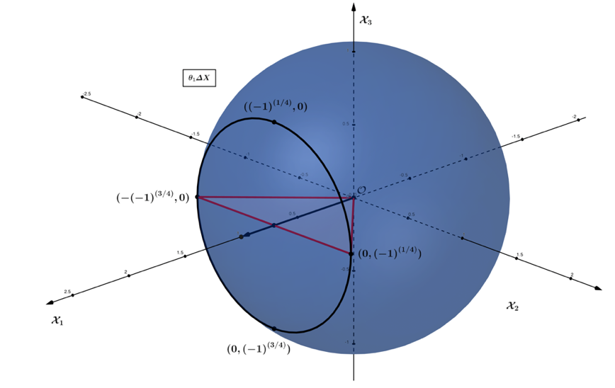
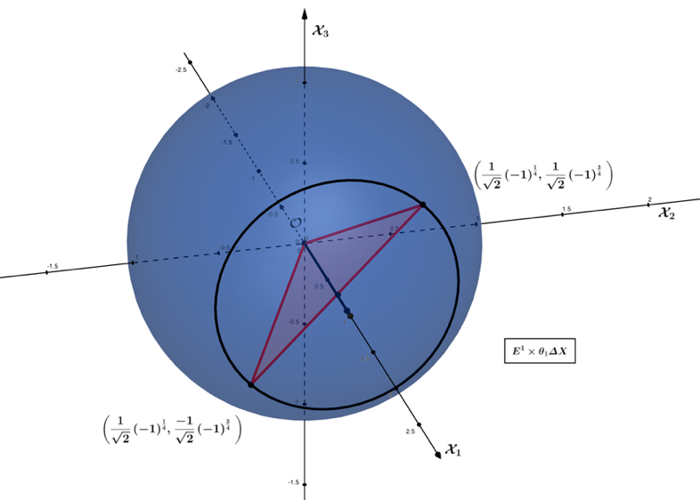
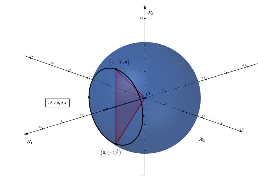
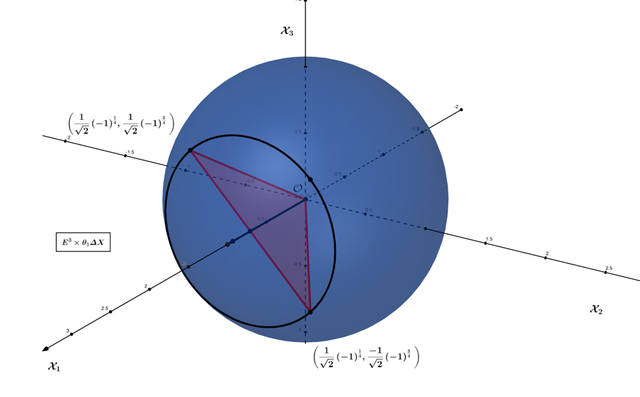
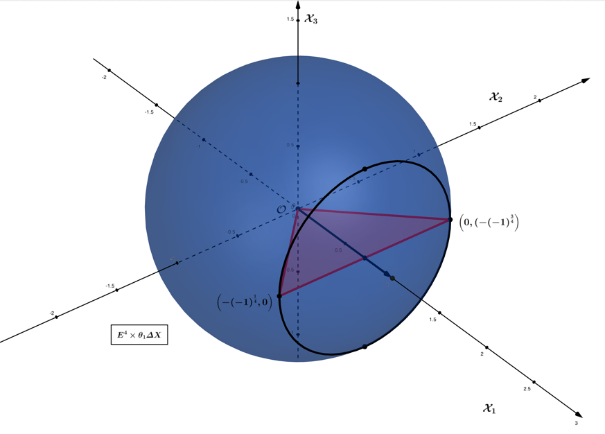
From the rotational iterations above, the evidence that a full revolution around the cone tangent space has occurred, comes by way of the return to the starting element at . One way to consider the graphical representation of the rotating -element, is by the following series of figures, where we start with the -element and proceed up to the rotation.
Figure 1.4.24 - Tangent Space Element as Polygonal Form.
Figure 1.4.25.a – Tangent Space Rotation
Figure 1.4.25.b – Tangent Space Rotation
Figure 1.4.26.a – Tangent Space Rotation
Figure 1.4.26.b – Tangent Space Rotation
By the rotation represented in Figure 1.4.26b, we have arrived at the negative form of our initial -element, which is discerned by the vector's arrowhead as compared to the -element (Figure 1.4.24). The figures represent the rotational axis , as fixed, but when looking at the iterations , the axis of rotation also moves along the unit circle. The result of this dynamic axis is that we have antipodal vector representations of all elements in the tangent space. The elements generated from the -rotations are very similar to those elements which generate the Lie algebra. We pursue this similarity, by evaluating products of the -elements, where we omit the angle variable , to represent similar forms to those of the elements
(1.4.199)
In the following products of the -elements, the bottom-right submatrices hold to the form, while the axis entry rotates in the axial-plane
(1.4.200)
The name assignment for these matrix products , is based on the bottom-right submatrices. The axes entries remain unchanged if considering the commutation operation of two elements . We can also see the antipodal relationships by considering that the vector elements are respectively antipodal to the elements . The matrix products of antipodal elements can be seen to generate the Lie algebras
(1.4.201)
To generalize the concept of antipodal elements, we represent the phase shift radians, from the previous rotation matrix , by using the mapping,
(1.4.202)
Returning to the -rotation matrix, we find its determinant equals
(1.4.203)
for which, we see that any element -cone tangent space has a determinant of , since Setting , the determinant simplifies to
(1.4.204)
where the volume of the -tangent space ring is simply , and for the case of our -rotations, for , we find that .
Next, would like to consider the divergence and curl of the -matrix. To do this we can decompose into its symmetric, , and antisymmetric, , parts
(1.4.205)
where
(1.4.206)
The diagonal matrix has a trace representative of the divergence of the -matrix group, while represents the curl-like antisymmetric portion of the -matrix group
(1.4.207)
(1.4.208)
The symmetric matrix is now trace-free
(1.4.209)
and we can express , as
(1.4.210)
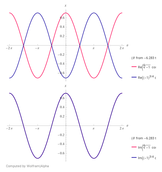
Concerning the curl matrix , a rotation is present, matching the circular ring that traces out the -cone tangent space, and is as expected. For the divergence matrix , setting, , and then plotting the cosine functions, reveals real values radians out of phase, and tandem in-phase superimposed imaginary values/waves, seen in the figure below.
Figure 1.4.27 – Divergence of the -cone tangent element, real-valued top,
(blue),(red), and imaginary-valued bottom.
Intuitively, the meaning of the divergence matrix
(1.4.211)
is that the divergence oscillates back and forth by in the -plane, by in the -plane, and by in the -plane. Setting , as we did in the determinant example, we find that the - plane diverges by , the -plane by , and the -plane by Taking the modulus of each of these complex values yields, and , which make intuitive sense since the moduli of the -plane values are a distance of away from the -axis. If we were to redefine our -plane rotation matrix, , to
(1.4.212)
the rotation axis would now be real-valued, admitting all values , and the -matrix determinant becomes
(1.4.213)
We consider the Cartesian equation of the infinite cone
(1.4.214)
whose parametric form can be found by solving for
then letting
(1.4.215)
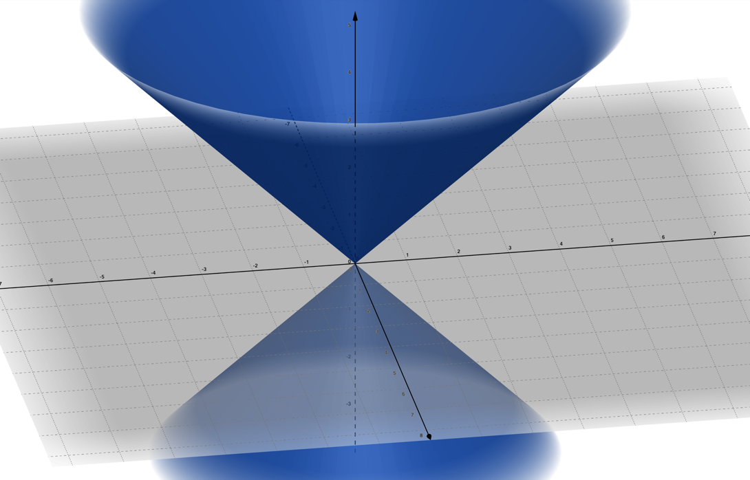
So, by setting , and defining, , the resulting equation represents the infinite Cartesian unit cone, plotted in Figure 1.4.28
(1.4.215)
Figure 1.4.28 – The infinite Cartesian unit cone, .
Concerning the infinite cone matrix group, an important distinction to make is for non-zero values, the cone will not come to a zero point at the center, and once the -matrix is exponentiated into the group-like form, there will be a non-zero geometric sphere at the center, which remains in the tangent space. An example would be to set , which yields the following determinant for
(1.4.216)
and the define , the result is
(1.4.217)
For all values , the infinite cone equation above gives the result , which is , and for values less than zero, approaches zero only as Although the form is algebraically correct, the same variable is present in all the components, and its path will travel equal in magnitude portions of the real and imaginary forms on the cone. The product of the -matrix and , yields a matrix group product , which encompasses both variables
(1.4.218)
By taking the determinant of , it can be seen clearly that this is the product of the unit hyperbola and the unit circle
(1.4.219)
Since , we can express the result of the determinant, as
(1.4.220)
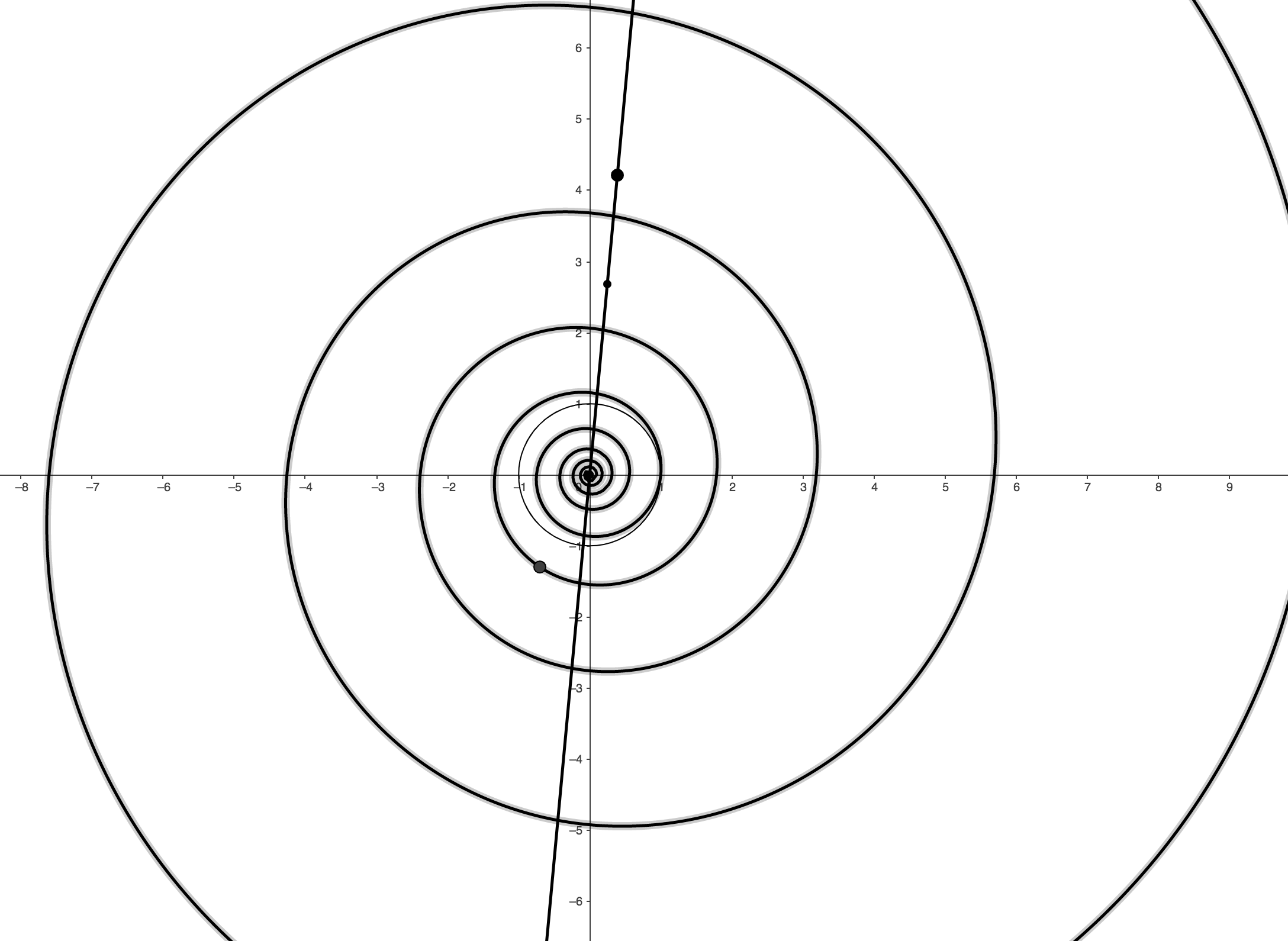
The function can be considered in terms of its real-valued component, representing the magnitude of the function along the real -axis and the imaginary-valued component as the circular rotation in the -plane. We can consider this determinant value as a non-axis number for , which is consistent with its cone number definition. To visually consider the determinant, we plot in Figure 1.4.29 the function , where the -plane is coming out of the page, and the - plane is the two-dimensional representation of the flat page. For larger values of the real component , we would see an increased distance between the arms of the spirals on the cone and, for smaller values of , tightly packed spirals on the cone would occur.
Figure 1.4.29 – Spirals on the cone of the function .
So far, we have been considering the cone section for the -plane. The representations are similar for the cone sections in the and -planes, which trace out circular tangent paths in the respective ,-planes. Similar representations are generated for the -plane cone, as
(1.4.221)
and the -plane cone, as
(1.4.222)
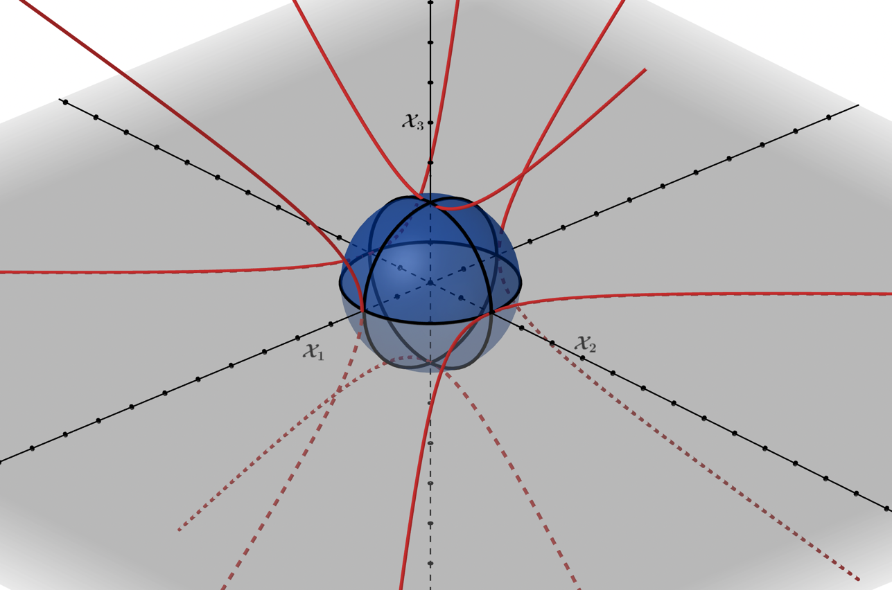
The unit sphere at the center of the conic is easily visualized as the intersection of three circular rings, representing the complex unit circle in its three orthogonal planes . This sphere is the group representation. In terms of the matrix group conic's hyperbolae, we can envision them as the result of each unit circle being opened and reflected from the imaginary axes to the real axes in the -planes, by way of a change in eccentricity. The hyperbolic analog to the -sphere is composed of unit hyperbolae, as three convexly oriented hyperbolic curves in each plane, facing away from the origin in the positive and negative directions. In Figure 1.4.30, we graph the geometric arrangement of the unit circles and unit hyperbolae with respect to one another.
Figure 1.4.30 – Centered tangent sphere at the origin, with intersecting unit circles on its surface,
and the unit hyperbolae intersecting the sphere atin the- planes.
Mathematically, the hyperbola represents an open and extended geometric curve, while the sphere is closed and non-extended. The cone can then be thought of as the perfect balance between the open and closed geometries of the circle and hyperbola in . We can envision it as the perfect balance between the sphere and the hypergeometry of the six-dimensional unit hyperbolae.
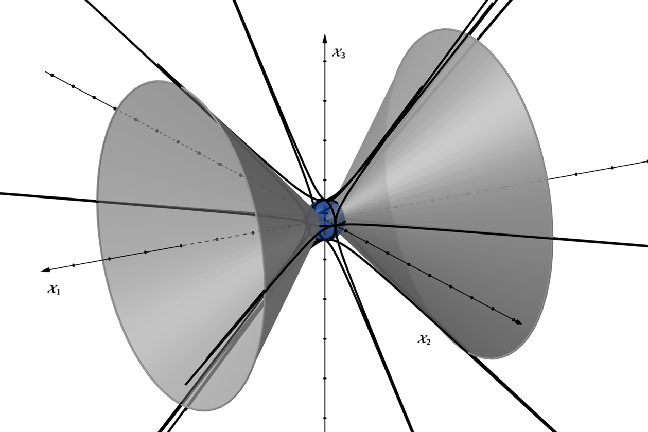
Figure 1.4.31 – The -cone oriented in relation to the tangent sphere, the six-dimensional
unit hyperbola and the six-dimensional complex unit sphere.
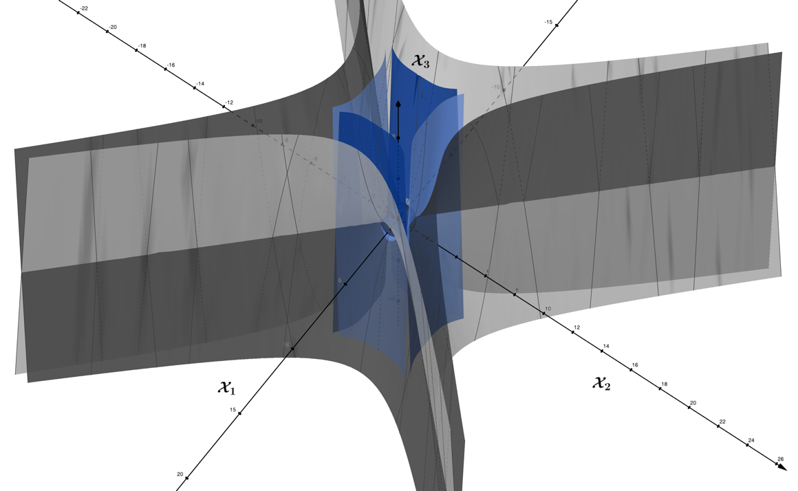
In Figure 1.4.31, we plot the -infinite unit cone, oriented in relationship to the hyperbolic and spherical geometries. The cones represent the asymptotic boundaries of the hyperbolae, which only approach this boundary at infinity. For the geometries extending beyond the unit invariant lengths, we plot the cone and the hyperbola in the - plane, Figure 1.4.32, where blue represents the -cone group, grey, the -hyperbola, and dark grey, the tangent sphere centered at the origin.
Figure 1.4.32 – -plane hyperbola and cone groups with non-invariant radial lengths.
The matrix group conic sections become extended through the exponential mapping of the tangent spaces on the surface of the sphere. The tangent sphere is the matrix group representation of a singularity situated at the origin, which contains all the information of the matrix groups, conveyed by the Lie algebra's information on its surface. Mathematically, values are bound to the various geometries that arise with the group exponentiation of Lie algebras and these values can be bound to certain subgroups of the group. An example of this would be boundedness on the six-dimensional hyperbolae , which arises from the matrix exponentiation of the Lie algebra, where boosts can elicit movement in the extended subspace of the real numbers, but this occurs in a distinct subspace of the matrix group conic sections.