It is essential to gain an intuitive grasp of how infinitesimal rotations of the equilateral triangle might occur. Using the example for our exponentiated element , and recalling that this permutation reflects the points and of the equilateral triangle about an axis passing through the point , which splits the triangle into equal halves. The generator acts on the identity element , and has the matrix-vector product representation
(1.1.124)
where for clarity, the angle of rotation is . The resulting matrix identity-vector product rotates the vertex around the unit circle in the -plane by , while the vertices are rotating in the -planes by . The rotation for the vertex around its fixed geodesic is the same rotation of a point around the complex unit circle like the case, and, as such, the group is embedded in the generator by default. Since the rotation of the vertices in the -plane may be less intuitive; we can consider it further in two different ways. The first is to follow the real and imaginary vector components of the respective vertices individually by taking each and -plane separately. To consider this geometrically, we set , to then calculate our matrix-vector product as
(1.1.125)
and gathering like vertex components by respective planes, we have
(1.1.126)
(1.1.127)
(1.1.128)
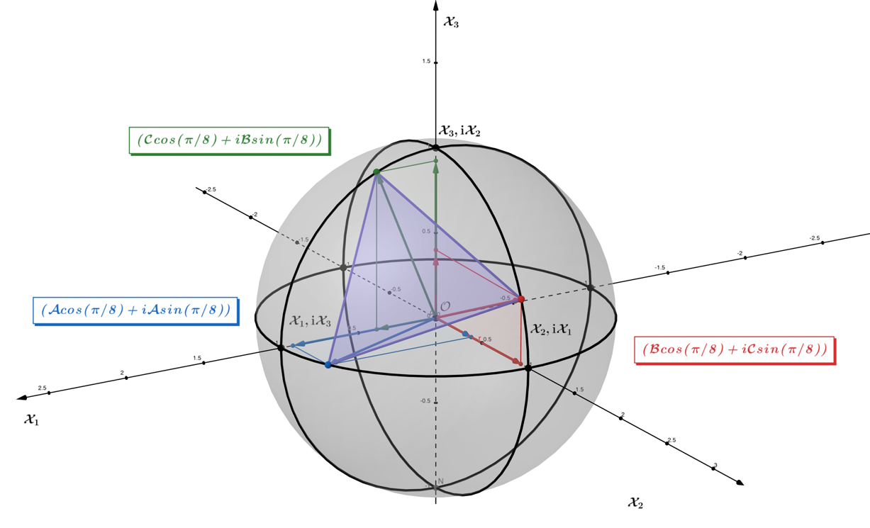
Figure 1.1.12 – for vectors.
In Figure 1.1.12, we graph these vectors, seeing that they maintain the polygonal form of the equilateral triangle, pictured in blue, with rotating vertices on the sphere's surface. The relationship in Eq. 1.1.25 is the result of taking the identity to be equal to the following matrix
(1.1.129)
and becomes
(1.1.130)
where each column represents the respective axis vector. When considering the matrix generator acting on a vector by left multiplication, performing a singular value decomposition of the matrix can give us a better idea of what steps happen to make this rotation occur. The reader can refer to Section 1.1.8 to review the SVD of a matrix if needed. As is diagonalizable, we take our to be a matrix with the eigenvalues along the diagonal, and our unitary matrices, , are just the eigenvectors arranged as columns in the matrix, coinciding with the respective entries in . The SVD can then be expressed as
(1.1.131)
where are
(1.1.132)
Above the eigenvectors in are normalized, and is equal to its conjugate transpose . Setting our identity vector to , for , choosing an angle value , and then calculating the product , we find
(1.1.133)
This shows that is taken to , the origin is taken to be , and that the vertex remains unchanged . Since are unitary in magnitude, the two-norm of the resulting vector is the same as the identity vector's two-norm , where both are equal to
(1.1.134)
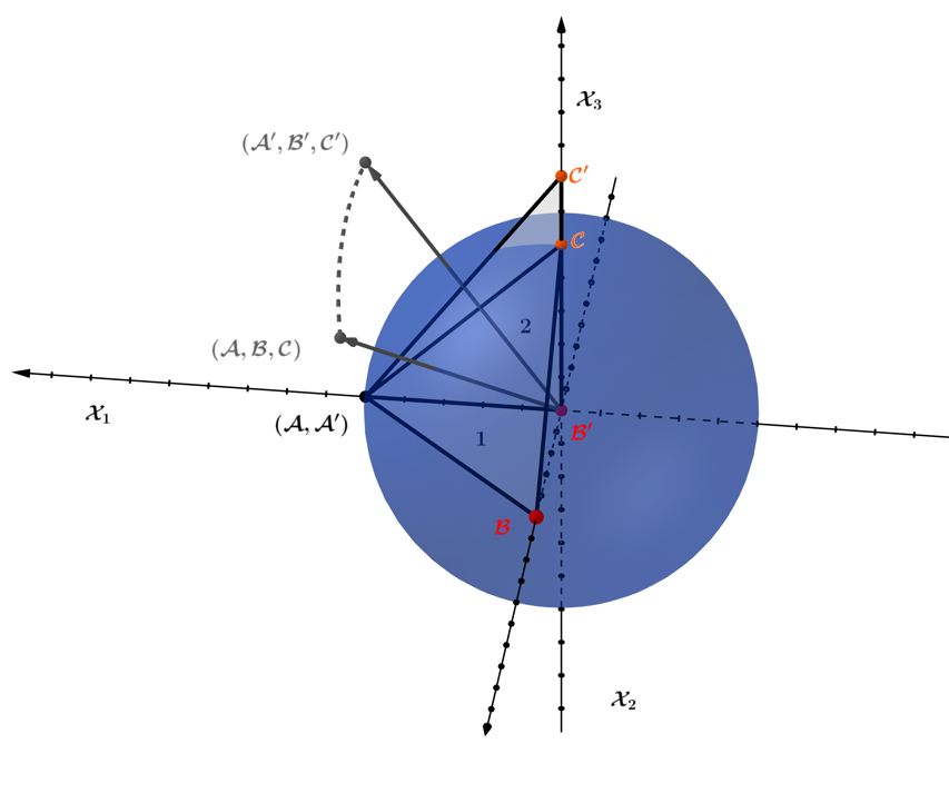
For our case, the two-norm is the magnitude of a vector with components , representing the coordinate values of the triangle's vertices in the -planes respectively. So, the result of is to rotate this triangle, whose vertices represent a vector , with an initial vector starting position , to the coordinates . The rotation of the triangle and its vector representation resulting from , is depicted in Figure 1.1.13, in which the starting triangle- with vertex coordinates has the vector representation depicted as , which both rotate as the result of the product to the triangle-, depicted at coordinates , along with the resulting vector representation This is consistent with what is the expected outcome from the portion of the SVD, which acts to rotate the vector/triangle by rotating the sphere.
Figure 1.1.13 – The rotation of the triangle and its vector representation .
The next step of the SVD is left multiplication by the matrix on the vector, which yields the vector
(1.1.135)
Given that is a diagonalized matrix of the eigenvalues of , the matrix-vector product scales , and accordingly, its geometric triangle/vector representations. As the eigenvalues are complex and unitary, the vector is rotated and scaled, as opposed to solely the scaling seen for a -matrix composed of real eigenvalues.
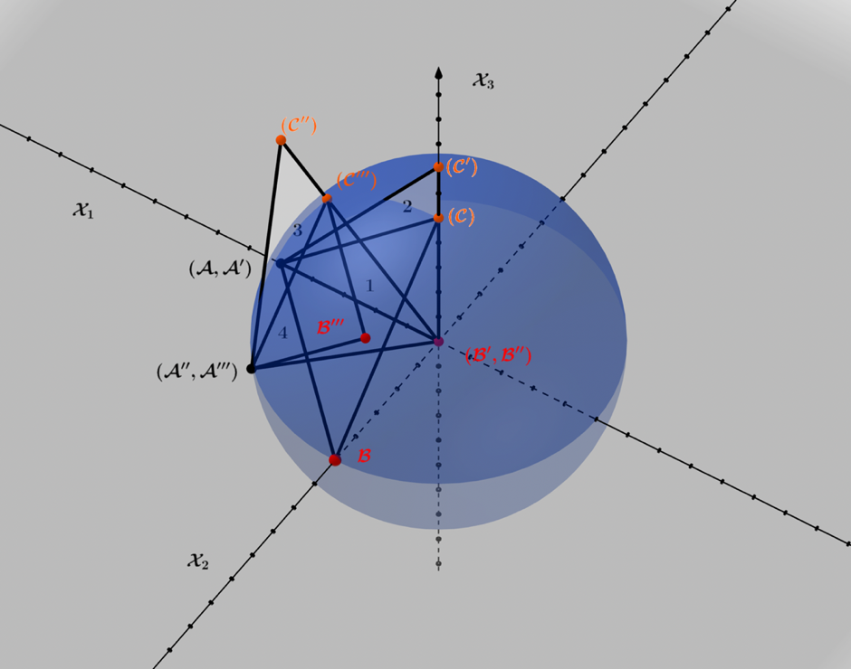
Figure 1.1.14 – The SVD decomposition of ,: triangle-,:
triangle-2,: triangle-3,: triangle-4.
In Figure 1.1.14, we track the path of the initial vector points , representing the triangle's vertices through the SVD decomposition The matrix-vector product brings us to the ultimate vector result, .
(1.1.136)
representing the linear transformation of the vector, the result of the matrix-vector product .