1.6.7 Transformations and Representation Theory

The Fouri­er trans­form rep­re­sents the means to de­ter­mine the an­gu­lar fre­quen­cy com­po­nents and or wavenum­ber com­po­nents of a wave­func­tion/signal. The Fouri­er trans­form in­volves mul­ti­ply­ing a func­tion by an ex­po­nen­tial series and then in­te­grat­ing the result, making it pos­si­ble to trans­form from the time and space do­mains to that of the fre­quen­cy domain and wave domain re­spec­tive­ly. We in­di­cate trans­formed func­tions with a hat above the func­tion and use $T,X,$for time-based and space-based func­tions. For a Fouri­er trans­form of a time-based wave­func­tion to the fre­quen­cy domain, the math­e­mat­i­cal rep­re­sen­ta­tion is

and the trans­form from the space-domain to the wave domain,

The reader's at­ten­tion should be di­rect­ed to the change in vari­able above from time to fre­quen­cy$\ (t \rightarrow f)$, from po­si­tion to wavenum­ber $(x \rightarrow k)$, and that the Fouri­er trans­form takes the in­verse of the wave­form units used for the re­sult­ing trans­form. Recall that fre­quen­cy is the in­verse of a wave's period, $f = T^{- 1}$, and sim­i­lar­ly for the wavenum­ber, there is an in­verse re­la­tion­ship to the wave­length, $k = \frac{2\pi}{\lambda}.$

Just as we can trans­form a wave­form from the time and space do­mains to the Fouri­er domain, an in­verse trans­form will bring us from Fouri­er domain back into the time and space do­mains. Using sim­i­lar no­ta­tion to the above Fouri­er trans­forms, the in­verse trans­forms for time/space-do­mains are

and

For these Fouri­er trans­forms to be an­a­lyt­ic, we re­quire that the in­te­grals are con­ver­gent and that the trans­formed wave­forms are con­tin­u­ous. To demon­strate, we take the ex­am­ple for the Fouri­er trans­form of the wave­form $X(x) = cos(2\pi k_{0}x)$, where

con­tin­u­ing, we take the Fouri­er trans­form $X(x) = sin(2\pi k_{0}x)$, find­ing

Adding the two cal­cu­lat­ed trans­forms from above, we find

for $\delta\left( k + k_{0} \right)$, the Dirac delta func­tion, and by taking its in­verse trans­form, Euler's for­mu­la is the ex­pect­ed result

This gives us a Fouri­er domain rep­re­sen­ta­tion com­posed of Dirac delta func­tions, which war­rants fur­ther dis­cus­sion. The Dirac delta func­tion is a rep­re­sen­ta­tion of a unit im­pulse, which equals zero for all values except $k = 0$, and this func­tion is typ­i­cal­ly taken to rep­re­sent the unit im­pulse of a point charge in physics. The func­tion at zero is in­fi­nite­ly narrow and in­fi­nite­ly tall, where the in­te­gral of the func­tion is equal to one, and math­e­mat­i­cal­ly, it is de­fined, as

with an in­te­gral equal to unity,

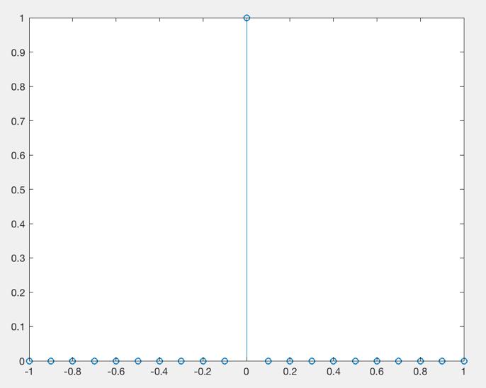
A plot of the Dirac delta func­tion $\delta(k)$, is shown in Figure 1.6.19, where it should be clear to see that the func­tion is equal to zero every­where except for a line at $k = 0$, which rises to in­fin­i­ty.

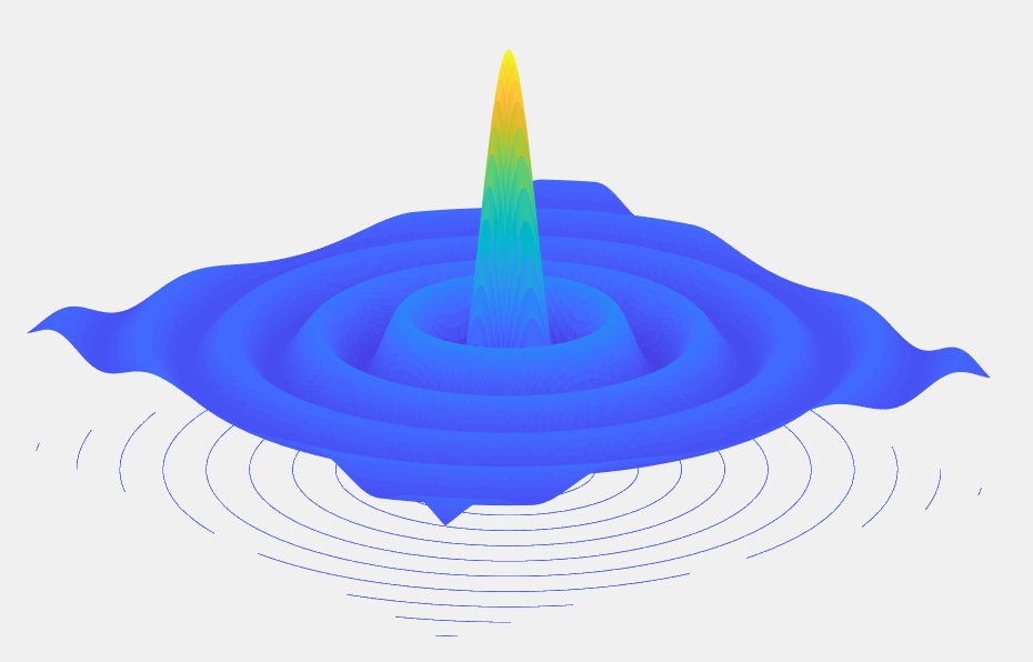
Re­turn­ing to the Fouri­er trans­form from the pre­vi­ous ex­am­ple, $\widehat{X}(k) = cos\left( 2\pi k_{0}x \right) = \frac{1}{2}\left( \delta\left( k - k_{0} \right) + \delta\left( k + k_{0} \right) \right)$, we see that it is com­prised of two im­puls­es in the Fouri­er domain that are non-zero only for $k = \pm k_{0}.$The fact that an in­fi­nite trigono­met­ric series can be sim­pli­fied into im­pulse spikes in the Fouri­er domain is pro­found. This spike is anal­o­gous to the im­pulse cre­at­ed by a pebble hit­ting the sur­face of an undis­turbed body of water, and the cir­cu­lar waves em­a­nat­ing away from the im­pulse would rep­re­sent its in­verse Fouri­er trans­form, de­pict­ed as a sur­face plot for the sinc func­tion, in Figure 1.6.20.

The sinc func­tion, also known as the sine car­di­nal func­tion, is fre­quent­ly used in signal pro­cess­ing and Fouri­er trans­form theory to rep­re­sent these unit im­puls­es, rep­re­sent­ed as

which is close­ly re­lat­ed to the spher­i­cal Bessel func­tion of the first kind,

The spher­i­cal Bessel func­tion of the first kind is re­lat­ed to the Bessel func­tion of the first kind, by

for $v,z\in \mathbb{C}$, and $J_{\left( v + \frac{1}{2} \right)}$, the Bessel func­tion of the first kind. Eval­u­at­ing the fol­low­ing in­te­gral

re­sults in the sinc func­tion, which in its nor­mal­ized form can be rep­re­sent­ed, as

and by taking its limit as $x \rightarrow \infty$, it equals unity

For the func­tion $asinc(fa)$, when taking the limit, as $a \rightarrow \infty,$it be­comes in­fin­i­ty at $f = 0$, making it clear that the ini­tial in­te­gral equals the Dirac delta func­tion with in­te­gra­tion bounds of neg­a­tive to pos­i­tive in­fin­i­ty

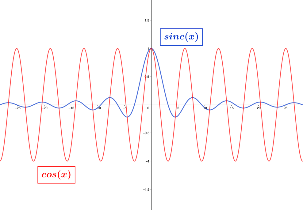
At­ten­tion should be di­rect­ed to the re­la­tion­ship be­tween the sinc and cosine func­tions, by plot­ting the two func­tions in Figure 1.6.21 below, where both equal $1$ at $x = 0$, and the peaks and troughs of the sinc func­tion, rep­re­sent­ing its local ex­trema, cor­re­spond with in­ter­sec­tion points on the cosine func­tion's wave­form.

From the in­tu­itive stand­point, the in­te­gral of a si­nu­soid over in­fi­nite time in both di­rec­tions is equal to zero, except for $f = 0$, when $\sin(0) = 0$, but at the same time, $\cos(0) = 1$, yield­ing an in­fi­nite in­te­gral at this point.

In Lie theory we typ­i­cal­ly con­sid­er the ex­po­nen­ti­at­ed group forms as a trans­for­ma­tion of the tan­gent space by way of the ex­po­nen­tial map­ping of its Lie al­ge­bra. When we con­sid­er in­fi­nite in­te­gra­tion as a con­tin­u­um in the coun­ter­clock­wise and clock­wise di­rec­tions, pre­vi­ous­ly stated as

we see in re­la­tion to Fouri­er trans­forms, that the in­fi­nite spike em­bod­ied in the Dirac delta and sinc func­tions is re­lat­ed to the iden­ti­ty el­e­ment sit­u­at­ed at $\left( \frac{e^{0 \times i\mathcal{a}_{m}}r^{0}}{0!} \right)$. Taking the de­riv­a­tive of a Lie group rep­re­sen­ta­tion with its vari­able equal to zero yields that group's Lie al­ge­bra, and this process is re­liant on the even trigono­met­ric func­tions of the group's de­riv­a­tive. Much the same occurs when taking the in­verse Fouri­er trans­form of a wave func­tion, which has its root in the in­fi­nite spikes co­in­cid­ing with the even cosine func­tion. We use an ex­am­ple to il­lus­trate a Dirac delta rep­re­sen­ta­tion for the prod­uct of two matrix groups from the in­fi­nite sym­me­try group $S_{3\mathbb{C}}^{\infty}$

Mul­ti­ply­ing the left and right sides by the $X,Y$ in­te­gra­tion op­er­a­tors, we find the fol­low­ing matrix that rep­re­sents the prod­uct of sinc func­tions

Taking the limit, as $a,b \rightarrow \infty$ for the re­spec­tive sinc func­tions in the matrix above re­sults in a matrix with the fol­low­ing prod­uct of Dirac delta func­tions

In our ex­am­ple, when taking double in­te­grals over time, the matrix en­tries with sine func­tions will become zero, while those with cosine func­tions will become sinc func­tions since $\cos{(0) = 1}$. The re­sult­ing delta matrix shows us that the trans­formed matrix group is the prod­uct com­po­si­tion of two matrix groups, $X_{1},X_{2}$

and much like in Fouri­er analy­sis, with its com­po­si­tion of si­nu­soids, the matrix group wave gen­er­a­tors of Lie theory and the $S_{3\mathbb{C}}^{\infty}$ sin­gu­lar­i­ty can be com­po­si­tions of matrix groups.

We have seen the link that in­fi­nite in­te­gra­tion has with ex­po­nen­ti­a­tion, and when con­sid­er­ing delta im­puls­es being in­te­grat­ed over in­fini­ties with Fouri­er trans­for­ma­tions, it is anal­o­gous to how the ex­po­nen­tial map­ping trans­forms a Lie al­ge­bra. To demon­strate this con­cept, a Lie al­ge­bra can be stated in terms of the Dirac delta dis­tri­b­u­tion func­tion, as

where $\left( k + k_{0} \right)$, de­notes the im­puls­es which are lo­cat­ed a dis­tance $k_{0}$ from the origin, and we typ­i­cal­ly set $k_{0} = 1$, to co­in­cide with our uni­tary study ap­proach. Mind­ful of this, for the Fouri­er trans­form, we have that

but the matrix rep­re­sen­ta­tion would differ as a higher-di­men­sion­al form $\in \mathbb{C}^{3}$, rep­re­sent­ing a ro­tat­ing equi­lat­er­al tri­an­gle in the $X_{2},X_{3}$-plane with an $X_{1}$-axis el­e­ment. The in­te­gra­tion op­er­a­tor that we pre­sent­ed ear­li­er acts to parse the delta func­tions from the lower right $2 \times 2$ matrix ro­ta­tion subset into cosine and sine func­tions

which yields the in­fi­nite in­te­gra­tion $f_{\mathbb{C}}^{- n}\left( X_{1} \right)$, ex­pressed using the in­fi­nite in­te­gra­tion op­er­a­tor ${\psi\left( X_{1} \right)}^{- n( - \infty,\infty)}$

The cen­tral tenet what we are con­sid­er­ing is that a deep con­nec­tion exists be­tween rep­re­sen­ta­tion theory and the Fouri­er trans­form. The im­puls­es in the tan­gent and sub­tan­gent spaces of the sin­gu­lar­i­ty trans­form into wave­forms in the ex­tend­ed space. The Baker-Camp­bell-Haus­dorff for­mu­la tells us that the prod­uct of two matrix groups is con­nect­ed to a Lie al­ge­bra that is part of the tan­gent space and com­posed of Lie brack­ets. These Lie al­ge­bras are rep­re­sen­ta­tion theory's ana­logue to the im­puls­es of Dirac delta dis­tri­b­u­tion for­mu­la.

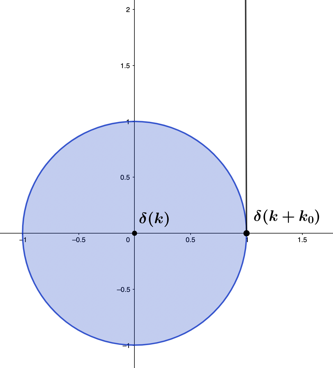
When con­sid­er­ing the sin­gu­lar­i­ty, we will need to expand our notion of the trans­for­ma­tion of the delta func­tion from an ori­en­ta­tion along the real-axis, to one that ori­ents not only on the com­plex unit circle but any­where on the com­plex unit sphere $\in \mathbb{C}^{3}$ space. This means that for any delta rep­re­sen­ta­tion $\delta\left( k + k_{0} \right)$, $k_{0}$ is not $\in \mathbb{R}$, but in­stead $k_{0}\in \mathbb{C}$, and fur­ther, $k_{0}$ is ori­ent­ed some­where in the higher di­men­sion­al­i­ty of the three com­plex planes $X_{1},X_{2},X_{3}$. The typ­i­cal treat­ment of the Dirac delta func­tion for $k_{0}\in \mathbb{R}$, is shown in Figure 1.6.22, where an in­fi­nite­ly narrow line, rooted at $k_{0} = 1,$goes off to in­fin­i­ty for $\delta\left( k + k_{0} \right)$.

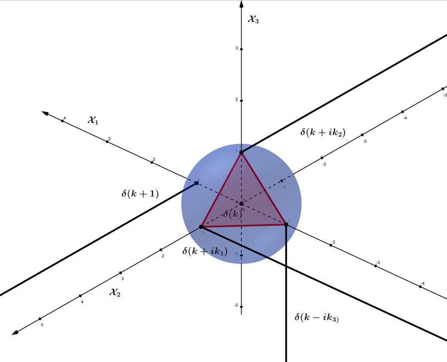
To demon­strate delta im­puls­es on the sin­gu­lar­i­ty in $\mathbb{C}^{3}$ space, we con­sid­er the equi­lat­er­al tri­an­gle sit­u­at­ed with ver­tices on the sin­gu­lar­i­ty's bound­ary, de­not­ing the delta func­tion $\in \mathbb{C}^{3}$, by $\delta\left( k + \left( k_{1},k_{2},k_{3} \right) \right)$, for $k_{j}$, the lo­ca­tions of each vertex in the $X_{1},X_{2},X_{3}$-planes re­spec­tive­ly. Chos­ing $k_{1} = i,\ k_{2} = i,\ k_{3} = - i$, we plot the com­plex spher­i­cal delta func­tion in Figure 1.6.23, for which, the reader's at­ten­tion should be drawn to the ori­en­ta­tion of the delta im­pulse lines from var­i­ous points on the sin­gu­lar­i­ty.

De­f­i­n­i­tion (1.6.239) – The Spher­i­cal Delta Func­tion is the rep­re­sen­ta­tion of the Dirac delta func­tion in $m$-di­men­sion­al com­plex space $\mathbb{C}^{m}$, de­not­ed as $\delta^{z}\left( \mu + \mu_{j} \right)$, where there are $m$ vari­ables for $\mu_{j}$, which is the dis­tance from the origin for each polyg­o­nal vertex in com­plex space, and $\mu_{j}$ can rep­re­sent space, time, wavenum­ber, or a fre­quen­cy rep­re­sen­ta­tion. For $m = 1$ and $\mu_{1}\in \mathbb{R}$, the spher­i­cal delta func­tion re­duces to the Dirac delta func­tion $\delta\left( \mu + \mu_{1} \right).$

The im­puls­es of the com­plex spher­i­cal delta func­tion em­anate tan­gen­tial­ly from the sin­gu­lar­i­ty's bound­ary from each of the ver­tices and this cor­re­sponds well with the treat­ment of the tan­gent space in Lie theory. The trans­la­tion of the spher­i­cal delta func­tion into its Lie al­ge­bra rep­re­sen­ta­tion is straight­for­ward when we con­sid­er that the delta func­tion $\delta(k + 1)$ is equal to the iden­ti­ty for $\delta\left( k + k_{0} \right)$, when $k_{0} = 1$. In­te­grat­ing the delta func­tion over neg­a­tive to pos­i­tive in­fin­i­ty

we know, based on the delta func­tion, is equal to zero every­where except at $k_{0} = 1$, where it is pos­i­tive in­fin­i­ty in value

An ex­pres­sion for the re­la­tion­ship of the spher­i­cal delta func­tion to its Lie al­ge­bra in the in­fi­nite sym­me­try group $\mathfrak{s}_{3\mathbb{C}}^{\infty}$, is stated as

which can be de­not­ed using our in­te­gra­tion op­er­a­tor no­ta­tion

The Lie al­ge­bra $\mathfrak{s}_{3\mathbb{C}}^{\infty}$ of the in­fi­nite sym­me­try group takes on com­plex-valued ex­po­nents, where real-valued ex­po­nen­tials will not nec­es­sar­i­ly have pe­ri­od­ic­i­ty akin to wave­forms, and this is based on the ec­cen­tric­i­ty of the geom­e­try we are con­sid­er­ing. To ad­dress this, in the up­com­ing book Phe­nom­e­nol­o­gy and the Geom­e­try of Light, we will study the use of the Laplace trans­form to ensure math­e­mat­i­cal con­sis­ten­cy with Lie theory. The Laplace trans­form is stated as

with a trans­form vari­able $s\in \mathbb{C}$, mean­ing it can take both real and imag­i­nary number values, en­com­pass­ing the math­e­mat­i­cal frame­work nec­es­sary for the trans­for­ma­tions of the com­plex spher­i­cal delta func­tion. The reader should be mind­ful that when taking the Laplace trans­form of a wave func­tion, it will simply reduce to the Fouri­er trans­form.