In conic sections, the cone is typically not given much thought and is considered as null, but when viewed as being a group in complex space, we start to see its importance, given other geometries arise from it. When talking about the set in the previous section, the tangent spaces of the individual exponential function points on the cone comprise the chord matrices of the form . The reader can recall that a tangent space is determined by the following calculation
(1.4.49)
and using our previous chord points , we denote them as unit equations
(1.4.50)
Calculating the tangent spaces of the above equations, we find
(1.4.51)
(1.4.52)
(1.4.53)
(1.4.54)
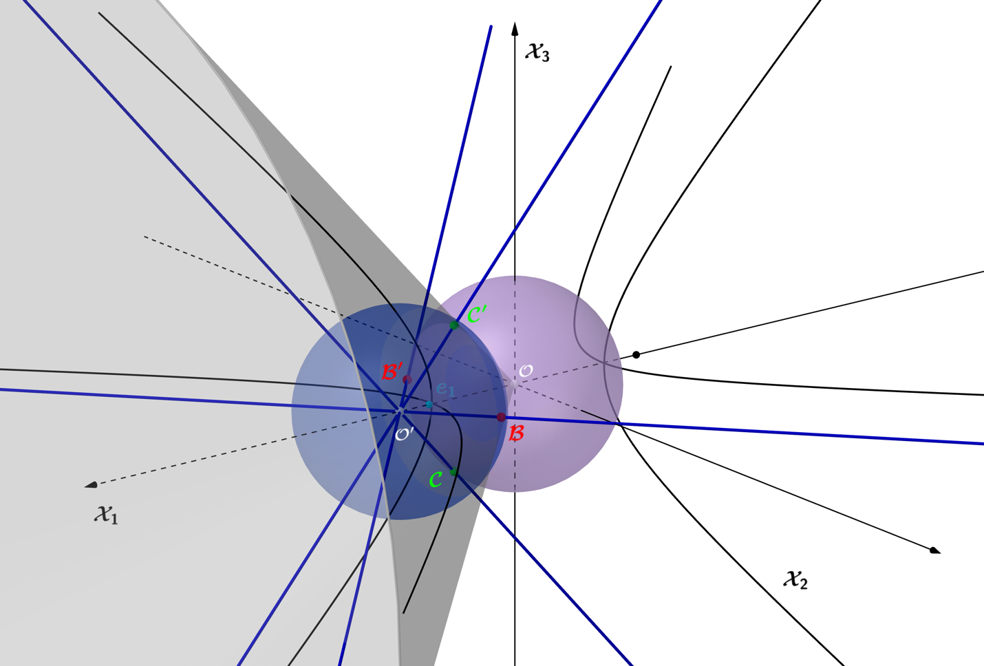
and we can see that the tangent spaces for our unit functions intersect the sphere exactly at the points . The tangent spaces meet at a confluence which is the focal point of the positive unit hyperbolae in the and -planes, and this confluence also forms the center of the inscribed sphere. In Figure 1.4.8, blue lines represent the tangent spaces for points intersecting at the point , which is the hyperbolic focal point and center of the inscribed sphere. The tangent points are intersection points on the sphere, seen in the figure for the inscribed sphere, and the cone oriented along the positive -axis.
Figure 1.4.8 – Tangent spaces as blue lines, meet at the point , the focal
point for the positive unit hyperbolae in the-plane, and the center of the inscribedsphere.
The tangent spaces for our matrix equations will continue to orient along points asymptotic to the unit hyperbola, based on increases in the magnitude of their arguments, forming the cones that bound the hyperbolae and the inscribed spheres. To show this, we take the matrix equation at the point , with a scalar constant , in the argument
(1.4.55)
for , the angle in radians, and calculate the tangent space of ,, finding
(1.4.56)
remarking that its tangent spaces simply scale by the constant,. Chord matrices for the scaled tangent spaces would then take the form for our original matrices, but would be scaled by a factor of , defining the radial distance to the points from the origin
(1.4.57)
The matrix elements calculate to
(1.4.58)
and the scaled group simply becomes
(1.4.59)
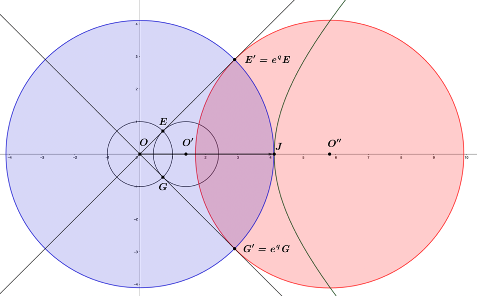
Figure 1.4.9 – Slice of -plane for the scaled inscribed sphere, for , and for , the center of the scaled sphere.
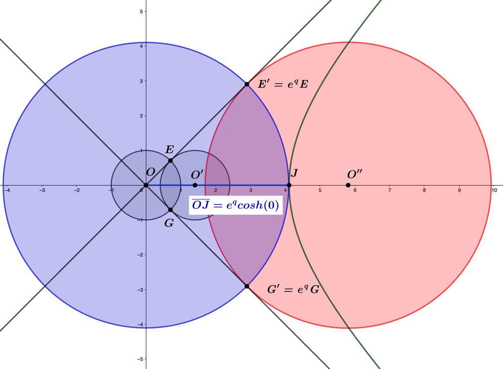
In Figure 1.4.9, we scale the inscribed sphere by the value , and take a slice of this along the -plane. The radial distance to the points is the new center point of the scaled inscribed sphere is located at , and the scaled inscribed sphere meets the cone at points . As the inscribed sphere increases in size, the unit hyperbola and the sphere scale by the same factor of (Figure 1.4.10).
Figure 1.4.10 – Slice of -plane for the scaled inscribed sphere for scaled unit sphere
with origin at, and scaled unit hyperbola with focal point at, and segment,.
The inscribed sphere of the scaled group will always have its origin at the coordinates, (, for those inscribed spheres centered along the -axis, with similar axis-based positions for spheres oriented about the other axes.