1.3.3 Vector Representations in Complex-Angled Space

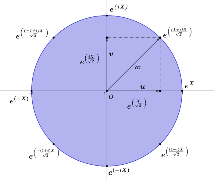
The polar vi­su­al­iza­tion of the com­plex unit circle nicely en­com­pass­es that a radial vector is a com­po­si­tion of an imag­i­nary-valued sine func­tion and a real-value cosine func­tion, ori­ent­ed re­spec­tive­ly along the ver­ti­cal and hor­i­zon­tal axes. A sim­i­lar geo­met­ric vi­su­al­iza­tion is pos­si­ble for the di­he­dral Lie groups using radial vector values to rep­re­sent a unique Lie group on the bound­ary $\partial \mathrm{B}$ of the com­plex-angle space. The com­po­nents of this radial vector stem from the imag­i­nary ex­po­nen­tial func­tion's con­tri­bu­tion along the ver­ti­cal axis and the real ex­po­nen­tial func­tion's con­tri­bu­tion along the hor­i­zon­tal axis (Figure 1.3.9).

Above, the vector $u$ rep­re­sents the real-valued ex­po­nen­tial func­tion $e^{\left( \frac{X}{\sqrt{2}} \right)}$, the vector $v$, the imag­i­nary-valued ex­po­nen­tial func­tion $e^{\left( \frac{iX}{\sqrt{2}} \right)}$, and the prod­uct of the two vector func­tions $u \bullet v$, re­sults in the ex­po­nen­tial func­tion $w$, that lies on the bound­ary of the disc

This simple case for a two-di­men­sion­al rep­re­sen­ta­tion holds for the di­he­dral Lie group gen­er­a­tors. Taking a sim­i­lar ex­am­ple in $\mathbb{C}^{3}$ space, the prod­uct of the ex­po­nen­tial func­tion vec­tors yields

which has the matrix rep­re­sen­ta­tion form

Con­sid­er­ing higher-di­men­sion­al tan­gent spaces using vector rep­re­sen­ta­tions proves useful for their geo­met­ric vi­su­al­iza­tion. We take the two gen­er­a­tors on the left-hand side of the equa­tion above, which have tan­gent space rep­re­sen­ta­tions found through the matrix log­a­rithm func­tion

We eval­u­at­ed the prod­uct of these func­tion vec­tors for the case with ex­po­nen­tial func­tion gen­er­a­tors, but given that the log­a­rithm func­tion yields the tan­gent vec­tors of the Lie groups, the tan­gent space on the bound­ary of our com­plex-angle spac**e, $\partial \mathrm{B}^{3\mathbb{C}}$, is the result of vector ad­di­tion

Ex­pand­ing the ad­di­tion of the tan­gent space vec­tors above, we find

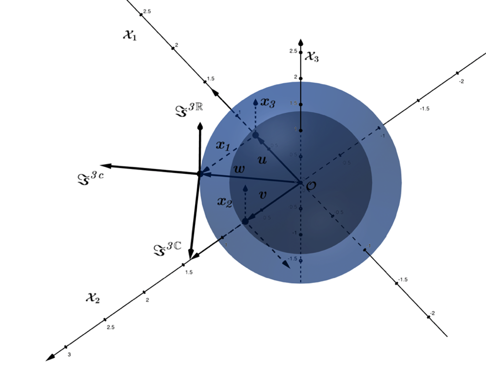
This is shown in Figure 1.3.10 for the two tan­gent spaces $\mathfrak{T}^{3\mathbb{C}}\left( \frac{X_{1}}{\sqrt{2}} \right)$, $\mathfrak{T}^{3\mathbb{R}}\left( \frac{X_{1}}{\sqrt{2}} \right)$, em­a­nat­ing from points on a sphere of radius $r = \frac{1}{\sqrt{2}}$. The vector ad­di­tion of these tan­gent spaces re­sults in the tan­gent space $\mathfrak{T}^{3\mathbb{c}}\left( X_{1} \right)$, which sits on the bound­ary of the com­plex-angle space $\partial \mathrm{B}^{3\mathbb{C}}$, a sphere of uni­tary mod­u­lus. La­beled on the $\mathfrak{T}^{3\mathbb{c}}\left( X_{1} \right)$ tan­gent space are the com­po­nent vec­tors $x_{1},x_{2},x_{3}$. These com­po­nent vec­tors reveal that $x_{1}$ stays in the plane of the ge­o­des­ic circle $e^{ix}$ for all tan­gent spaces $\mathfrak{T}^{3\mathbb{C}}\left( \frac{X_{1}}{\sqrt{2}} \right),\mathfrak{T}^{3\mathbb{R}}\left( \frac{X_{1}}{\sqrt{2}} \right),\ \mathfrak{T}^{3\mathbb{c}}\left( X_{1} \right)$, while main­tain­ing an or­thog­o­nal re­la­tion­ship to the sphere's bound­ary along its ge­o­des­ic path. This con­trasts with the vec­tors $x_{2},x_{3}$, which orient along the $X_{3}$,$\ X_{2}$-axes re­spec­tive­ly, and always main­tain an or­thog­o­nal ori­en­ta­tion to their proper $X_{2},X_{3}$-axes. These ori­en­ta­tions and re­la­tions should make sense, re­call­ing that the $X_{1}$ el­e­ment in the $D_{3}$ di­he­dral group re­flects the two points $B,C\ (x_{2},x_{3})$, leav­ing the point $A\left( x_{1} \right)$ fixed.